Fabian Gröger    Shuo Wen    Maria Brbić

Abstract

The Platonic Representation Hypothesis suggests that representations from neural networks are converging to a common statistical model of reality. We show that the existing metrics used to measure representational similarity are confounded by network scale: increasing model depth or width can systematically inflate representational similarity scores. To correct these effects, we introduce a permutation-based null-calibration framework that transforms any representational similarity metric into a calibrated score with statistical guarantees. We revisit the Platonic Representation Hypothesis with our calibration framework, which reveals a nuanced picture: the apparent convergence reported by global spectral measures largely disappears after calibration, while local neighborhood similarity, but not local distances, retains significant agreement across different modalities. Based on these findings, we propose the Aristotelian Representation Hypothesis: representations in neural networks are converging to shared local neighborhood relationships.

Platonic Representation Hypothesis, Representation Similarity, Hypothesis Testing, Representation Learning, Unsupervised Learning,

1 Introduction

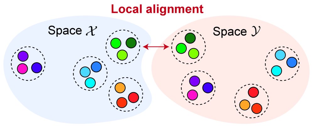
Figure 1: The Aristotelian Representation Hypothesis: Local relations (“who is near whom”), rather than distances between data points, are preserved across different representation spaces. Representation learning algorithms will converge to shared local neighborhood relationships.

Quantifying the similarity between neural network representations is central to understanding the geometry of learned representation spaces ^{1 2}, guiding transfer learning decisions ^{3 4}, and relating artificial representations to neural measurements in neuroscience ⁵. The Platonic Representation Hypothesis ⁶ posits that as neural networks scale, representations across different modalities become increasingly similar, suggesting convergence to a shared statistical model of reality. This hypothesis has motivated a growing literature that uses representational similarity to study whether scaling produces universal structure across models ^{6 7 8 9}. To measure representational similarity across models, different metrics have been proposed, such as Centered Kernel Alignment ³, Canonical Correlation Analysis ¹⁰, Representational Similarity Analysis ¹¹, and mutual $k$ -Nearest Neighbors ⁶.

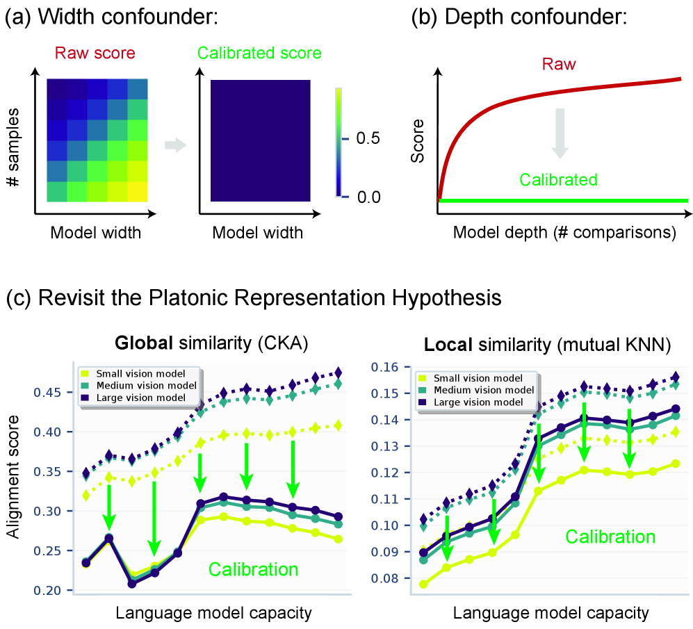
Figure 2: Null calibration removes width and depth confounders. (a) Width confounder: raw scores exhibit positive null baselines that increase with the ratio of dimension (width) of the spaces and the number of samples; calibration collapses them to zero. (b) Depth confounder: selection-based summaries (max over layers) inflate with search space size; aggregation-aware calibration removes this. (c) After calibration, global metrics lose their convergence trend, while local metrics retain significant alignment.

In this work, we identify two pervasive confounders that distort representational similarity measurements. The first is the model width: when the embedding dimension increases relative to the sample size, interaction-matrix-based similarity metrics exhibit a systematic positive baseline even when representations are independent. This spurious similarity is a general consequence of dimensionality-driven null inflation: the expected similarity under independence does not vanish but instead depends on both the representation dimensionality and the sample size (Figure 2a). As a result, wider models can appear more aligned simply because their representations live in higher-dimensional spaces. The second confounder is the model depth. Many analyses do not compare individual layer pairs, because it is unknown where similarity arises ^{5 6}. Instead, they search over all pairs and report a summary statistic such as the maximum. Taking a maximum over many comparisons inflates the reported score even if there is no similarity, since the expected maximum of independent draws exceeds the mean. This inflation grows with the number of comparisons, so deeper models can appear more aligned simply because more layer pairs are compared (Figure 2b). Together, these confounders undermine the comparative use of representational similarity without calibration.

To address these issues, we introduce the null-calibration for representational similarity, a general permutation-based framework that transforms any similarity metric into a calibrated score with a principled null reference, here defined as no relationship (Figure 2). The core idea is to measure how extreme an observed similarity is relative to an empirical null distribution obtained by breaking sample correspondences. For scalar comparisons (i.e., width confounder), we estimate a critical threshold from the null distribution and define a calibrated score that is zero when the observed similarity falls below this threshold and rescaled to preserve the maximum at one. For selection-based summaries (i.e., depth confounder), we apply aggregation-aware calibration. We compute the null distribution of the same aggregate statistic that is ultimately reported (e.g., the maximum over all layer pairs), thereby calibrating the selection step itself.

These observations raise a question: Does the Platonic Representation Hypothesis still hold once similarity is calibrated? We find that, after calibration, the previously reported convergence in global metrics ^{6 7 8} largely disappears, suggesting it was driven primarily by width and depth confounders, whereas local neighborhood-based metrics retain significant cross-modal alignment (Figure 2c). However, we also observe that the convergence in local distances is not preserved, suggesting that only local neighborhood relationships are aligned. Motivated by these results, we refine the original Platonic Representation Hypothesis and propose the Aristotelian Representation Hypothesis ¹: Neural networks, trained with different objectives on different data and modalities, converge to shared local neighborhood relationships (Figure 1). We name it after the Greek philosopher Aristotle, who was a student of Plato and, in his Categories, established the principles of relatives ¹².

2 Related work

Representational similarity metrics.

A long line of work compares representation spaces using a variety of similarity measures. Canonical Correlation Analysis (CCA) ¹³ and variants such as Singular Vector Canonical Correlation Analysis (SVCCA) ¹ and Projection Weighted Canonical Correlation Analysis (PWCCA) ¹⁴ compare subspaces up to linear transformations, while Procrustes- and shape-based distances compare representations up to restricted alignment classes ^{15 16}. Centered Kernel Alignment (CKA) ³ has become a dominant tool for comparing deep representations, with kernelized variants extending to nonlinear similarity. Representational Similarity Analysis (RSA) ¹¹, originating in neuroscience, compares representational dissimilarity matrices rather than feature bases. Neighborhood-based approaches, such as mutual $k$ -Nearest Neighbors (mKNN) ⁶, capture local topological consistency rather than global alignment. However, recent evaluations stress that different metrics encode different invariances and can yield qualitatively different conclusions, motivating more robust reporting practices ^{17 15 18 19}.

Reliability of representational similarity metrics.

In finite-sample, high-dimensional regimes, raw similarity scores can be systematically biased. Recent works ^{20 21} propose debiased CKA, but these corrections are metric-specific. For neighborhood-based metrics, no analogous debiasing methods exist despite distance concentration effects that inflate random k-NN overlap ^{22 23}. Other approaches address confounding from input population structure. For instance, ²⁴ propose regression-style deconfounding to remove effects of shared input statistics on RSA / CKA. A separate reliability issue arises from layer search, where max or top- $k$ aggregation across many layer pairs introduces multiple-comparison inflation. While resampling-based “maxT” procedures ^{25 26} can calibrate such aggregates, this has not yet been applied in representational similarity studies. Our calibration framework addresses both finite-sample bias and selection inflation in a unified, metric-agnostic way.

The Platonic Representation Hypothesis.

A growing body of work examines whether neural networks trained under different conditions converge toward similar representations. The Platonic Representation Hypothesis ⁶ posits that as models scale, their representations increasingly converge across architectures and even across modalities such as vision and language, with convergence reported under both global and local similarity measures. Follow-up work has examined factors influencing these trends, including model size, training duration, and data distribution ²⁷, and has explored analogous convergence effects in broader settings such as video models ⁹ and comparisons to biological vision ²⁸. In this work, we revisit the Platonic Representation Hypothesis using our null-calibration framework that controls for width and depth confounders.

3 Problem setup

3.1 Representation spaces and similarity score

Let $\mathcal{X}\subseteq\mathbb{R}^{d_{x}}$ and $\mathcal{Y}\subseteq\mathbb{R}^{d_{y}}$ be two representation spaces, where $d_{x}$ and $d_{y}$ are the respective space dimensions. For a set of $n$ input samples, let $\mathbf{X}\in\mathbb{R}^{n\times d_{x}}$ and $\mathbf{Y}\in\mathbb{R}^{n\times d_{y}}$ be the corresponding embeddings in $\mathcal{X}$ and $\mathcal{Y}$. We assume row-wise alignment such that the $i$ -th row of $\mathbf{X}$ and $\mathbf{Y}$ correspond to paired inputs. We use a similarity score $s(\mathcal{X},\mathcal{Y})\in\mathbb{R}$ to quantify the agreement between $\mathcal{X}$ and $\mathcal{Y}$. In practice, we compute it from $\mathbf{X},\mathbf{Y}$ and, by a slight abuse of notation, denote it with $s(\mathbf{X},\mathbf{Y})$.

We consider a generic similarity function $s(\mathbf{X},\mathbf{Y})\in\mathbb{R}$. Our focus covers three families of metrics: (i) spectral: metrics defined on the spectrum of cross-covariance or Gram matrices (e.g., CKA, CCA), (ii) neighborhood: metrics measuring local topological overlap (e.g., mKNN), and (iii) geometric: second-order isomorphism metrics (e.g., RSA). Appendix C provides definitions of the metrics used in this paper.

3.2 The null hypothesis of independence

We claim that a similarity score $s(\mathbf{X},\mathbf{Y})$ is uninterpretable without a baseline. To provide this baseline, we define the null hypothesis $H_{0}$ as the absence of a relationship between $\mathbf{X}$ and $\mathbf{Y}$ beyond their marginal statistics. We operationalize $H_{0}$ via a permutation group $\Pi_{n}$ acting on sample indices: draw $\pi\sim\mathrm{Unif}(\Pi_{n})$ independently of $(\mathbf{X},\mathbf{Y})$ and evaluate $s(\mathbf{X},\pi(\mathbf{Y}))$, where $\pi(\mathbf{Y})$ permutes the rows of $\mathbf{Y}$.

Assumption 3.1 (Exchangeability under the null).

Under $H_{0}$, the joint distribution of paired samples is invariant to relabeling of correspondences. For any permutation $\pi\in\Pi_{n}$, $\mathbb{P}{H{0}}(\mathbf{X},\mathbf{Y})=\mathbb{P}{H{0}}(\mathbf{X},\pi(\mathbf{Y}))$.

This assumption implies that if no true relationship exists, the observed pairing is statistically indistinguishable from a random shuffling of the data. It allows us to construct an empirical null distribution by holding $\mathbf{X}$ fixed and shuffling the rows of $\mathbf{Y}$.

3.3 Baseline problem: non-zero null expectations

Ideally, under $H_{0}$, we desire $\mathbb{E}_{\pi}[s(\mathbf{X},\pi(\mathbf{Y}))]\approx 0$. However, for commonly used raw or biased estimators, the expected similarity under the null is not zero,

\[\mu_{0}(n,d_{x},d_{y})\,\coloneqq\,\mathbb{E}_{\pi}[s(\mathbf{X},\pi(\mathbf{Y}))].\]

This baseline $\mu_{0}$ is metric- and preprocessing-dependent and can deviate from zero in finite samples. It also varies with sample size and dimension, thus acting as a confounding variable in comparative studies.

4 Theoretical motivation: spurious alignment

We motivate and formalize why raw representational similarity metrics fail in cross-scale model comparisons. We identify two distinct sources of confounding: (i) the width confounder driven by representation dimension, and (ii) the depth confounder driven by the number of layers considered when comparing models.

4.1 The width confounder

Many spectral-family similarity metrics, e.g., linear/kernel CKA, the RV coefficient, and CCA -based scores (CCA /SVCCA/PWCCA), can be written as functionals of an interaction operator constructed from two representations. One such operator is the (normalized) cross-covariance

\[\widetilde{\mathbf{C}}\;=\;\frac{1}{n-1}\mathbf{X}_{c}^{\top}\mathbf{Y}_{c}\in\mathbb{R}^{d_{x}\times d_{y}},\]

where $\mathbf{X}{c}$ and $\mathbf{Y}{c}$ denote row-centered representations (Section C.1).

A common but misleading intuition is that if $\mathbf{X}$ and $\mathbf{Y}$ are independent, then $\widetilde{\mathbf{C}}\approx\mathbf{0}$ and therefore spectral aggregates should be near zero. In high dimension this fails: the null interaction energy is typically non-zero.

Proposition 4.1 (Non-vanishing null interaction energy).

Assume the rows are i.i.d. with $\mathbb{E}[\mathbf{x}{i}]=\mathbb{E}[\mathbf{y}{i}]=0$, $\mathrm{Cov}(\mathbf{x}{i})=\mathbf{I}{d_{x}}$, $\mathrm{Cov}(\mathbf{y}{i})=\mathbf{I}{d_{y}}$, and $\mathbf{x}{i}$ and $\mathbf{y}{i}$ are independent. Then

\[\mathbb{E}_{H_{0}}\left[\|\widetilde{\mathbf{C}}\|_{F}^{2}\right]\;=\;\frac{d_{x}d_{y}}{n-1}.\]

Proof. See Section D.4.

Since CKA is scaled by the normalized self-similarity terms, which each scale as $\mathcal{O}(\sqrt{d})$, the resulting null baseline for the metric is thus $\mathcal{O}(d/n)$.

This aligns with insights from random matrix theory: in high-dimensional regimes ($d\sim n$), the null singular spectrum of interaction operators (after centering/whitening) concentrates into a non-trivial “noise bulk” whose upper edge depends on $d/n$ and preprocessing, rather than collapsing to zero ^{29 30}. Our framework estimates this null baseline directly via permutation, providing a metric- and pipeline-independent alternative to asymptotic formulas.

Neighborhood metrics follow a different regime.

While spectral metrics have null baselines scaling as $\mathcal{O}(d/n)$, neighborhood-based metrics such as mutual $k$ -NN exhibit different behavior, as they rely on set comparisons rather than interactions.

Proposition 4.2 (Null baseline for neighborhood metrics).

Assume the rows are i.i.d. with $\mathbf{x}{i}$ and $\mathbf{y}{i}$ independent, and that pairwise distances are almost surely distinct (e.g., under absolutely continuous distributions). Then for any $k<n$,

\[\mathbb{E}_{H_{0}}\bigg[\mathrm{mKNN}(\mathbf{X},\mathbf{Y})\bigg]\;=\;\frac{k}{n-1}.\]

Proof. See Section D.6.

In particular, neighborhood metrics have null baselines scaling as $\mathcal{O}(k/n)$.

The difference in null baseline between spectral and neighborhood metrics is substantial: (i) The neighborhood scale $k$ can be fixed consistently across experiments, whereas the embedding dimension $d$ is determined by the model architecture, making it difficult to control in comparison studies. (ii) The neighborhood metrics are much less confounded since $k\ll d$ in typical settings.

4.2 The depth confounder

A subtle yet pervasive issue is the comparison of selection-based alignment summaries across models. Let $S_{\ell,\ell^{\prime}}:=s(\mathbf{X}^{(A)}{\ell},\mathbf{Y}^{(B)}{\ell^{\prime}})$ be the similarity between layer $\ell$ of model $A$ and layer $\ell^{\prime}$ of model $B$. It is common to summarize the similarity between two models by the maximum alignment score $T_{\max}=\max_{\ell,\ell^{\prime}}S_{\ell,\ell^{\prime}}$. Let $M=L_{A}L_{B}$ be the number of layer pairs searched, where $L_{A}$ and $L_{B}$ are the depths of models $A$ and $B$. Even under $H_{0}$, taking a maximum over $M$ comparisons inflates the reported score, a “look-elsewhere” effect. This is an instance of the classical multiple comparisons problem ^{31 32}: as $M$ increases, the probability that at least one null similarity exceeds any fixed threshold grows, inflating the expected maximum. Consequently, when alignment is summarized via a max or top- $k$ statistic without correction, unrelated representations can exhibit spuriously high reported similarity, as the inflation depends on model depth, making raw summaries non-comparable across architectures.

Characterizing this inflation does not require independence across pairs. It follows from a uniform right-tail bound. Assume there exist a common mean $\mu\in\mathbb{R}$ and $\sigma>0$ such that the null fluctuations satisfy, for all $(\ell,\ell^{\prime})$ and all $t\geq 0$,

\[\mathbb{P}(S_{\ell,\ell^{\prime}}-\mu\geq t)\leq\exp\!\left(-\frac{t^{2}}{2\sigma^{2}}\right).\]

For bounded similarities $S_{\ell,\ell^{\prime}}\in[s_{\min},s_{\max}]$, Hoeffding’s inequality implies a sub-Gaussian right-tail bound of the form Equation 5 with $\sigma\leq(s_{\max}-s_{\min})/2$. This covers many common bounded metrics (e.g., CKA / RSA / mKNN). Crucially, only the right tail is needed for bounding the maximum. Then a union bound gives

\[\mathbb{P}(T_{\max}-\mu\geq t)\leq M\exp\!\left(-\frac{t^{2}}{2\sigma^{2}}\right),\]

and consequently for a constant $C$

\[\mathbb{E}_{H_{0}}\left[T_{\max}\right]\;\leq\;\mu+C\,\sigma\sqrt{\log M}.\]

Proof. See Section D.5.

This creates a depth confounder. Deeper models (larger $M=L_{A}L_{B}$) can attain higher raw “max-alignment” scores purely because of a larger search space. Correlations across neighboring layers reduce the effective number of comparisons, but the inflation remains monotone in the search space size in typical workflows. Therefore, raw scaling plots of $T_{\max}$ (or top- $k$ summaries) are not comparable across architectures unless the selection step itself is calibrated.

5 Representational similarity calibration

To overcome the issues of the width and depth confounders, we introduce the null-calibration for representational similarity. The key idea is to compare observed similarity scores against an empirical null distribution obtained by permuting sample correspondences, thereby establishing a principled zero point that accounts for finite-sample, high-dimensional artifacts.

5.1 Null-calibrated similarity

We propose null-calibrated similarity measures to correct for width and depth confounders by transforming raw similarity scores into an effect size with a principled zero point.

Given representations $\mathbf{X}\in\mathbb{R}^{n\times d_{x}}$ and $\mathbf{Y}\in\mathbb{R}^{n\times d_{y}}$ aligned by rows, we operationalize the null hypothesis $H_{0}$ (no relationship beyond marginal statistics) by permuting sample correspondences. For permutations $\pi_{k}\in\Pi_{n}$ drawn i.i.d. uniformly from $\Pi_{n}$ and independently of $(\mathbf{X},\mathbf{Y})$, we form null scores

\[s^{(k)}=s(\mathbf{X},\pi_{k}(\mathbf{Y})),\qquad k=1,\dots,K.\]

Let $s_{\mathrm{obs}}:=s(\mathbf{X},\mathbf{Y})$ denote the observed score. Let $s_{(1)}\leq s_{(2)}\leq\cdots\leq s_{(K+1)}$ denote the order statistics of the combined multiset ${s_{\mathrm{obs}},s^{(1)},\dots,s^{(K)}}$ (with ties allowed). We define a right-tail rank-based critical value:

\[\tau_{\alpha}\;:=\;s_{(\lceil(1-\alpha)(K+1)\rceil)},\]

where $\lceil(1-\alpha)(K+1)\rceil$ is the $(1-\alpha)$ -quantile of the $(K+1)$ -sized multiset and the empirical right-tail $p$ -value:

\[p\;=\;\frac{1+\#\{k\in\{1,\dots,K\}:s^{(k)}\geq s_{\mathrm{obs}}\}}{K+1}.\]

The critical value $\tau_{\alpha}$ defines a robust zero point: values below $\tau_{\alpha}$ are typical under $H_{0}$ at level $\alpha$, while $p$ provides an evidence measure that can be combined with multiple-testing correction when many comparisons are performed.

The proposed calibration framework relies on randomization (permutation) to construct a null distribution for any similarity statistic. This yields finite-sample guarantees under an exchangeability condition (Section 3.2), and it implies useful invariances that make calibrated scores comparable across metrics and implementations.

The permutation $p$ -value in Equation 10 is super-uniform under $H_{0}$ (i.e., $\mathbb{P}{H{0}}(p\leq\alpha)\leq\alpha$ for all $\alpha\in[0,1]$), a standard consequence of randomization inference ^{26 33 34} (see Section D.1 for formal definitions and proofs).

Corollary 5.1 (Type-I control for calibrated scores).

Let $s_{\mathrm{obs}}=s(\mathbf{X},\mathbf{Y})$ and $s^{(k)}=s(\mathbf{X},\pi_{k}(\mathbf{Y}))$ for $k=1,\dots,K$. Define the add-one permutation $p$ -value $p$ as in Equation 10, and equivalently define the rank-based critical value $\tau_{\alpha}:=s_{(\lceil(1-\alpha)(K+1)\rceil)}$ from the sorted combined set ${s_{\mathrm{obs}},s^{(1)},\dots,s^{(K)}}$. Under Section 3.2,

\[\mathbb{P}_{H_{0}}\big(p\leq\alpha\big)\leq\alpha\quad\text{and hence}\quad\mathbb{P}_{H_{0}}\big(s_{\mathrm{obs}}>\tau_{\alpha}\big)\leq\alpha,\]

so the gating rule “ $s_{\mathrm{cal}}>0$ ” (where $s_{\mathrm{cal}}$ is the calibrated score defined in Equation 12, which implies $p\leq\alpha$) is a finite-sample $\alpha$ -level declaration of similarity above chance.

Proof. Follows directly from Section D.1; see Section D.1.

Calibrated score (scalar case).

While $p$ -values and null percentiles are rank-based and therefore invariant under monotone transformations of the raw score (Section D.2; see Section D.2), effect sizes serve a complementary purpose: they quantify how much similarity exceeds chance on an interpretable scale. The calibrated score achieves this by rescaling the excess over the null threshold $\tau_{\alpha}$ to the interval $[0,1]$. This rescaling is not monotone-invariant, and this by design. A purely rank-based calibration would be equivalent to a score shift and would be unable to correct for the scale-dependent null baselines identified in Section 4. The calibrated score instead adapts to the actual null distribution, providing a meaningful zero point.

For bounded similarity metrics with known maximum $s_{\max}$ (often $s_{\max}=1$), we define a max-preserving calibrated score

\[s_{\mathrm{cal}}=\max\!\left(\frac{s_{\mathrm{obs}}-\tau_{\alpha}}{s_{\max}-\tau_{\alpha}},0\right).\]

This calibrated score depends on the chosen level $\alpha$ through $\tau_{\alpha}$ (Equation 9). We therefore also report the corresponding permutation $p$ -value and/or null percentile for an $\alpha$ -free summary. This score satisfies $s_{\mathrm{cal}}=0$ whenever $s_{\mathrm{obs}}\leq\tau_{\alpha}$ (i.e., below the estimated right-tail critical value of the permutation null), and $s_{\mathrm{cal}}=1$ when $s_{\mathrm{obs}}=s_{\max}$ (i.e., perfect similarity remains $1$). When $s_{\max}$ is unknown, or the metric is unbounded, we default to the unnormalized effect size $[s-\tau_{\alpha}]{+}=\max(s-\tau{\alpha},0)$.

5.2 Aggregation-aware null-calibration

To analyze the similarity between two models $A$ and $B$ with depths $L_{A}$ and $L_{B}$, a common approach is to compute a layer-by-layer similarity matrix $\mathbf{S}\in\mathbb{R}^{L_{A}\times L_{B}}$ by evaluating a similarity score for every pair of layers:

\[S_{\ell,\ell^{\prime}}=s\!\left(\mathbf{X}^{(A)}_{\ell},\mathbf{Y}^{(B)}_{\ell^{\prime}}\right),\]

where $\mathbf{X}^{(A)}{\ell}\in\mathbb{R}^{n\times d{\ell}}$ and $\mathbf{Y}^{(B)}{\ell^{\prime}}\in\mathbb{R}^{n\times d{\ell^{\prime}}}$ are the representations of models $A$ and $B$ at layers $\ell$ and $\ell^{\prime}$ respectively, evaluated on $n$ samples, and $s(\cdot,\cdot)$ is a similarity metric. A common practice is then to summarize $\mathbf{S}$ by a selection-based aggregation operator, such as taking the maximum. These summaries are attractive because they support statements such as “there exists a layer in $A$ that matches some layer in $B$ ” or “each layer of $A$ best matches a layer in $B$ ”. However, selection introduces a statistical effect: even under the null hypothesis of no relationship between representations, selection-based summaries are systematically inflated.

As analyzed in Section 4.2, this inflation grows with the number of layer pairs and makes naïve post-selection $p$ -values anti-conservative. Our aggregation-aware calibration addresses this by calibrating the reported statistic directly: the null distribution must match the entire analysis pipeline. Let the aggregate score be $T(\mathbf{S})$ (e.g., a maximum), then the appropriate null is the distribution of $T(\mathbf{S})$ under a valid null transformation (e.g., permuting sample correspondences). We therefore define an aggregation-aware permutation null.

Consistency of permutations across layers.

For each draw $\pi_{k}\in\Pi_{n}$, we apply the same sample permutation to all layers of model $B$ and define

\(\displaystyle S^{(k)}_{\ell,\ell^{\prime}}:=s\!\left(\mathbf{X}^{(A)}_{\ell},\pi_{k}\!\left(\mathbf{Y}^{(B)}_{\ell^{\prime}}\right)\right),\) \(\displaystyle\ell=1,\dots,L_{A},\quad\ell^{\prime}=1,\dots,L_{B},\)

then compute $T^{(k)}:=T(\mathbf{S}^{(k)})$. Let $T_{\mathrm{obs}}:=T(\mathbf{S})$ denote the observed aggregate. Let $T_{(1)}\leq\cdots\leq T_{(K+1)}$ denote the order statistics of the combined set ${T_{\mathrm{obs}},T^{(1)},\dots,T^{(K)}}$ (with ties allowed). We define

\[\tau_{\alpha}^{\mathrm{agg}}:=T_{(\lceil(1-\alpha)(K+1)\rceil)},\]

where $\lceil(1-\alpha)(K+1)\rceil$ is the $(1-\alpha)$ -quantile of the $(K+1)$ -sized multiset. We report the right-tail permutation $p$ -value

\[p_{\mathrm{agg}}=\frac{1+\#\{k\in\{1,\ldots,K\}:T^{(k)}\geq T_{\mathrm{obs}}\}}{K+1},\]

By the same exchangeability argument as for scalar calibration, $p_{\mathrm{agg}}$ is super-uniform under $H_{0}$ (see Section D.3).

Calibrated score (aggregate case).

For bounded similarities with maximum $s_{\max}$ (often $s_{\max}=1$), we report a max-preserving calibrated aggregate

\[T_{\mathrm{cal}}=\max\!\left(\frac{T_{\mathrm{obs}}-\tau_{\alpha}^{\mathrm{agg}}}{s_{\max}-\tau_{\alpha}^{\mathrm{agg}}},\,0\right).\]

This score satisfies $T_{\mathrm{cal}}=0$ when $T_{\mathrm{obs}}\leq\tau_{\alpha}^{\mathrm{agg}}$ and $T_{\mathrm{cal}}=1$ when $T_{\mathrm{obs}}=s_{\max}$. As above, $T_{\mathrm{cal}}$ depends on $\alpha$ via $\tau_{\alpha}^{\mathrm{agg}}$; we therefore report both $T_{\mathrm{cal}}$ (magnitude above null) and $p_{\mathrm{agg}}$ (evidence against null), applying multiplicity correction ^{35 31} when many model pairs are evaluated.

5.3 Summary

To compute a calibrated similarity score: (i) fix a significance level $\alpha$ (e.g., $\alpha=0.05$); (ii) generate $K$ null scores by permuting sample correspondences; (iii) compute critical value $\tau$ as the $\lceil(1-\alpha)(K+1)\rceil$ -th order statistic of the combined set (observed + null scores); (iv) return calibrated score, either $s_{\mathrm{cal}}$ or $T_{\mathrm{cal}}$.

Use scalar calibration (Section 5.1) when comparing a single pair of representations. Use aggregation-aware calibration (Section 5.2) when reporting a summary statistic (e.g., maximum) over multiple layer pairs. Appendix E provides pseudocode for both procedures.

6 Experiments

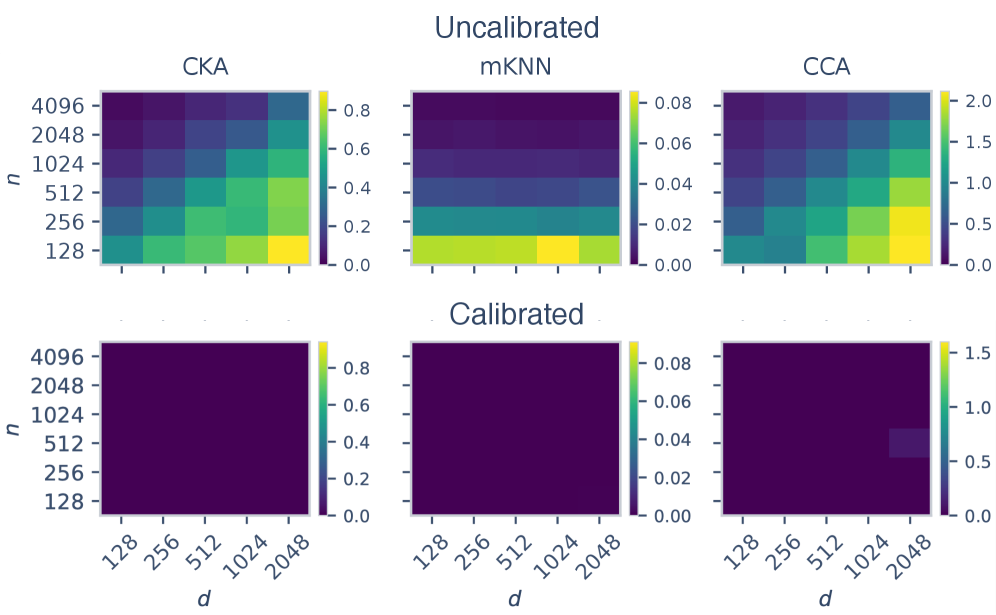
Figure 3: Calibration eliminates spurious similarity across metrics. Raw scores (top) drift with d / n d/n; calibrated scores (bottom) collapse to zero. Results for heavy-tailed distributions and additional metrics are in Section F.6.

We quantify the effects of the width and depth confounders in controlled synthetic experiments and show that our calibration framework effectively removes them. We then revisit the Platonic Representation Hypothesis using our calibration framework, assessing which convergence trends remain robust after controlling for these confounding factors.

6.1 Null-calibration removes width confounder

We validate that our calibration eliminates width-related inflation of similarity across metrics, regimes, and noise distributions, without metric-specific derivations.

We design controlled synthetic experiments as follows. Under $H_{0}$, we draw $\mathbf{X},\mathbf{Y}\in\mathbb{R}^{n\times d}$ independently from Gaussian and heavy-tailed (Student- $t$, Laplace) distributions. We sweep the number of samples $n\in{128,256,512,1024,2048,4096}$ and the dimension $d\in{128,256,512,1024,2048}$. Under $H_{1}$, we inject a shared low-rank signal component and vary the signal-to-noise ratio. We evaluate representative metrics spanning three families. For spectral similarity, we use linear and RBF CKA, as well as CCA /SVCCA/PWCCA; for neighborhood similarity, we use mKNN (with $k=10$); and for geometric similarities, we use RSA and Procrustes. Figure 3 reports a subset of these metrics for readability; additional metrics are reported in Section F.6. For calibration, we use $K=200$ permutations with $\alpha=0.05$.

Under $H_{0}$, uncalibrated scores increase with $d/n$, while our calibrated scores stay at zero across settings (Figure 3). This confirms that the similarity scores of wider models can arise purely from high-dimensional finite-sample effects, and our calibration removes this spurious baseline. Importantly, the magnitude of the null baseline is metric-dependent, consistent with our theory: CKA’s baseline scales as $\mathcal{O}(d/n)$ (Section 4.1), while mKNN ’s baseline scales as $\mathcal{O}(k/n)$ (Section 4.1). Intuitively, mKNN compares local neighborhood overlap at a fixed $k$, thus only comparing relationships instead of local distances, making its null baseline insensitive to representation width $d$, which explains the order-of-magnitude gap observed in raw scores. The same pattern holds for heavy-tailed noise (Section F.6).

Next, we verify the statistical guarantees of our empirical null calibration. For Type-I error control, rejection rates stay at or below the nominal $\alpha=0.05$ across $(n,d/n)$ configurations (Figure 4a). Crucially, our calibration does not sacrifice sensitivity to real alignment: detection rates increase rapidly with signal strength (Figure 4b). Overall, our calibration preserves signal structure: in the high-signal regime, raw and calibrated scores show the same pattern, while in the low-signal regime, calibration correctly gates scores to zero (Section F.2).

Furthermore, we verify that our empirical calibration closely matches existing analytical bias corrections for CKA ²⁰, recovering the width correction without metric-specific derivation (Section F.4).

Additionally, we perform ablations on different noise distributions used in the synthetic experiments (Section F.1), different calibration approaches (Section F.3), and an ablation on the influence of the number of permutations $K$ used for calibration (Section F.5).

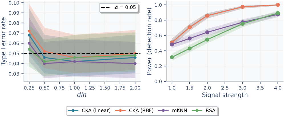
Figure 4: Statistical guarantees. (Left) Type-I error stays at or below α \alpha across configurations. (Right) Power increases rapidly with signal strength; calibration does not sacrifice sensitivity.

6.2 Null-calibration removes depth confounder

We validate that our aggregation-aware null-calibration eliminates the depth confounder. To build a controlled synthetic setting, we construct two synthetic models, $A$ and $B$, each with $L$ layers. Under $H_{0}$, we sample layer representations ${\mathbf{X}{\ell}}{\ell=1}^{L}$ and ${\mathbf{Y}{\ell^{\prime}}}{\ell^{\prime}=1}^{L}$, where each $\mathbf{X}{\ell},\mathbf{Y}{\ell^{\prime}}\in\mathbb{R}^{n\times d}$ has i.i.d. $\mathcal{N}(0,1)$ entries (independent across layers and between models), using $d/n=8$ to match the upper range of the Platonic Representation Hypothesis setting. We then compute the layerwise similarity matrix $S_{\ell,\ell^{\prime}}=\operatorname{CKA}{\text{lin}}(\mathbf{X}{\ell},\mathbf{Y}_{\ell^{\prime}})$ and summarize it with standard aggregation operators.

The uncalibrated max-aggregated scores inflate with layer count even under $H_{0}$ (Figure 5): raw max-scores are systematically higher at $L=128$ than at $L=1$, despite no true signal. Our aggregation-aware calibration eliminates this bias: calibrated aggregates remain stable regardless of depth. We further show that naively calibrating each scalar comparison still leads to inflation, highlighting the importance of calibrating the final statistic. Furthermore, since deeper models tend to be wider as well, raw comparisons are doubly confounded.

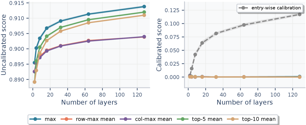
Figure 5: Aggregation-aware calibration removes depth confounding. Raw max-aggregates of linear CKA scores inflate with layer count under the null; calibrated aggregates are stable and show that naive entry-wise calibration still leads to inflation.

(a) CKA RBF: Global spectral alignment.

6.3 Revisiting the Platonic Representation Hypothesis

A central claim behind the Platonic Representation Hypothesis is that, as models become more capable, their representations begin to converge across modalities. We revisit this claim through our calibration framework to determine whether the observed alignment reflects genuine shared representation structure or instead arises from width and depth confounders.

We follow the experimental protocol of ⁶ using $n=1024$ image–text pairs (WIT; ³⁶) and embeddings from three language model families (Bloomz, OpenLLaMA, LLaMA) and five vision model families (ImageNet-21K, MAE, DINOv2, CLIP, CLIP-finetuned) across multiple scales. This yields 204 vision–language model pairs spanning $d/n\in[0.75,8]$. For each pair, we compute layer-wise similarity and report the maximum across layers, as in the original work. We evaluate both global spectral metrics (CKA linear/RBF) and local neighborhood metrics (mKNN, cycle- $k$ NN, CKNNA). Following ⁶, we evaluate mKNN, cycle- $k$ NN, and CKNNA with $k=10$. We further apply Benjamini-Hochberg FDR correction ³¹ to control for multiple comparisons across model pairs.

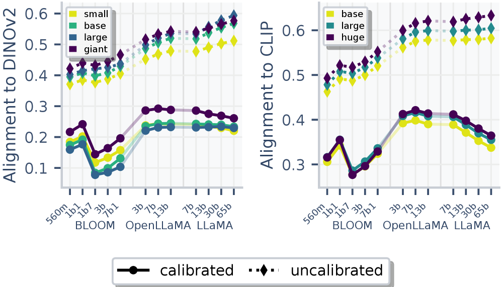
For the global similarity, we find that uncalibrated CKA scores increase with model scale (dotted lines in Figure 6a), reproducing the trend interpreted as evidence of cross-modal convergence ⁶. However, this trend disappears after our calibration (solid lines): calibrated CKA shows no systematic increase with model size. This indicates that global convergence in uncalibrated CKA is largely attributable to width and depth confounders rather than a genuine increase in representational similarity.

In contrast, for the local similarity, evidence of cross-modal convergence remains strong for neighborhood-based metrics even under our calibration (Figure 6b). The same qualitative conclusion holds for other neighborhood-based measures (cycle- $k$ NN and CKNNA; Section F.7) and different choices of $\alpha$ (Section F.10). Further analysis (Section F.9) reveals that models converge in local neighborhood structure: models increasingly agree on which points are neighbors, but do not agree on the pairwise distances, since CKA-RBF with a small bandwidth shows no alignment after calibration.

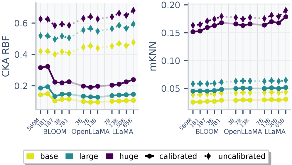
Figure 7: Video–language alignment. Extending the Platonic Representation Hypothesis analysis to video encoders (VideoMAE base/large/huge) yields the same pattern: calibrated CKA drops substantially while mKNN retains alignment.

To test whether these findings generalize beyond images and text, we extend our analysis to video–language alignment following ⁹. We compare video encoders (VideoMAE base/large/huge) against the same language model families. Consistent with our previous findings, the global similarity (CKA) shows no trend with model capacity (Figure 7). In contrast, for local similarity (mKNN), a clear scaling trend emerges with VideoMAE-Huge, whereas smaller video encoders appear to act as a bottleneck, limiting alignment regardless of language model size. This confirms that local neighborhood convergence extends to video–language alignment, provided that representations are sufficiently powerful. Section F.8 further compares a variety of image models at the frame level on the same dataset, showing the same trend.

Taken together, these results suggest a refined version of the Platonic Representation Hypothesis. After calibration, we find little evidence that representations converge in global spectral structure as models scale, at least under the considered setting. What reliably persists is local geometric alignment: different models preserve similar neighborhood relationships among inputs. We therefore propose the alternative Aristotelian Representation Hypothesis: As models become capable, their representations converge to shared local neighborhood relationships.

7 Conclusion

Representational similarity metrics are widely used to study learned features, but their interpretation is systematically distorted by two artifacts: width-dependent null baselines and depth-dependent selection inflation. We introduced a unified null-calibration framework that corrects both, turning similarity scores into effect sizes with principled zero points and valid $p$ -values. Applying our framework to the Platonic Representation Hypothesis reveals that previously reported global spectral convergence is largely confounded by width and depth, whereas local neighborhood alignment remains significant, motivating an Aristotelian Representation Hypothesis.

Acknowledgements

We thank Artyom Gadetsky, Siba Smarak Panigrahi, Debajyoti Dasgupta, David Frühbuss, Shin Matsushima, Rishubh Singh, Adriana Moreno Castan, and Gioele La Manno for their valuable suggestions, which helped improve the manuscript. We are especially grateful to Simone Lionetti for additional input and support. We gratefully acknowledge the support of the Swiss National Science Foundation (SNSF) starting grant TMSGI2_226252/1, SNSF grant IC00I0_231922, and the Swiss AI Initiative. M.B. is a CIFAR Fellow in the Multiscale Human Program.

References

Appendix A Limitations

Permutation calibration is finite-sample valid under Section 3.2, which treats the $n$ row pairs as exchangeable units. In practice, exchangeability can be violated even without a sequential structure (e.g., grouped/clustered samples). In such settings, validity is recovered by using restricted permutations that preserve the dependence structure (e.g., permuting within blocks or permuting block labels) and by re-running under each restricted permutation.

Appendix B Existing calibration approaches for representational similarity metrics

Table 1: Comparison of prior works. Y=yes, N=no, P=partial/indirect. “Debias” indicates an explicit null correction of the reported similarity. “Bounded” indicates whether the corrected score preserves an interpretable upper bound (e.g., 1 for perfect alignment). “Agg-aware” indicates calibration of selection-based aggregates (e.g., max over layer pairs).

Ref	Metric(s)	Debias?	Bounded?	Agg-aware?
20	CKA	Y	N	N
21	CKA	Y	N	N
24	RSA / CKA	P	N	N
37	RSA (cv/ WUC)	Y	P	N
38	RSA (Bayes)	P	N	N
39	RV / adj. RV	Y	N	N
Ours	Any bounded metric	Y	Y	Y

Appendix C Metrics and score definitions

This appendix gives the definitions of the similarity metrics $s(\mathbf{X},\mathbf{Y})$ used throughout the paper. The main text focuses on the calibration procedure (Sections 5 and 5.2). Here we provide concrete instantiations of the metrics referenced in Section 3 and Section 6.

C.1 Preprocessing and basic notation

Let $\mathbf{X}\in\mathbb{R}^{n\times d_{x}}$ and $\mathbf{Y}\in\mathbb{R}^{n\times d_{y}}$ denote row-aligned representations evaluated on the same $n$ inputs. We use the centering matrix

\[\mathbf{H}\;=\;\mathbf{I}_{n}-\frac{1}{n}\mathbbm{1}_{n}\mathbbm{1}_{n}^{\top},\]

where $\mathbf{I}{n}\in\mathbb{R}^{n\times n}$ is the identity matrix and $\mathbbm{1}{n}\in\mathbb{R}^{n}$ is the all-ones vector. We define row-centered representations $\mathbf{X}{c}=\mathbf{H}\mathbf{X}$ and $\mathbf{Y}{c}=\mathbf{H}\mathbf{Y}$. Unless stated otherwise, similarities are computed on centered representations.

C.2 Raw similarity metrics

This section provides formal definitions of the similarity metrics used throughout the paper. In the main text, we primarily use CKA (linear and RBF kernel) ³, RSA ¹¹, and mutual $k$ -NN ⁶ as representative metrics from the spectral, geometric, and neighborhood families, respectively. Additional metrics (SVCCA, PWCCA, cycle- $k$ NN, CKNNA, RV coefficient, Procrustes) are included for completeness and used in supplementary experiments.

C.2.1 Spectral metrics

Linear Centered Kernel Alignment (CKA).

Linear CKA ³ can be written as a normalized Frobenius energy of the sample cross-covariance operator. With $\mathbf{X}{c},\mathbf{Y}{c}$ as above, define the sample (cross-)covariances

\[\widetilde{\mathbf{\Sigma}}_{XX}:=\frac{1}{n-1}\mathbf{X}_{c}^{\top}\mathbf{X}_{c},\qquad\widetilde{\mathbf{\Sigma}}_{YY}:=\frac{1}{n-1}\mathbf{Y}_{c}^{\top}\mathbf{Y}_{c},\qquad\widetilde{\mathbf{C}}:=\widetilde{\mathbf{\Sigma}}_{XY}:=\frac{1}{n-1}\mathbf{X}_{c}^{\top}\mathbf{Y}_{c}.\]

The biased linear Hilbert-Schmidt Independence Criterion (HSIC) energy equals $|\widetilde{\mathbf{C}}|_{F}^{2}$. The commonly used linear CKA normalization can be written as

\[\mathrm{CKA}_{\mathrm{lin}}(\mathbf{X},\mathbf{Y})\;=\;\frac{\|\widetilde{\mathbf{C}}\|_{F}^{2}}{\|\widetilde{\mathbf{\Sigma}}_{XX}\|_{F}\,\|\widetilde{\mathbf{\Sigma}}_{YY}\|_{F}}\;=\;\frac{\|\mathbf{X}_{c}^{\top}\mathbf{Y}_{c}\|_{F}^{2}}{\|\mathbf{X}_{c}^{\top}\mathbf{X}_{c}\|_{F}\,\|\mathbf{Y}_{c}^{\top}\mathbf{Y}_{c}\|_{F}}\;\in\;[0,1],\]

where the second equality follows by cancellation of common $1/(n-1)$ factors.

Kernel Centered Kernel Alignment.

Kernel CKA ³ generalizes linear CKA by replacing dot products with kernel functions. Let $k_{X}:\mathbb{R}^{d_{x}}\times\mathbb{R}^{d_{x}}\to\mathbb{R}$ and $k_{Y}:\mathbb{R}^{d_{y}}\times\mathbb{R}^{d_{y}}\to\mathbb{R}$ be positive semidefinite kernel functions (e.g., RBF kernel $k_{X}(\mathbf{x},\mathbf{x}^{\prime})=\exp(-|\mathbf{x}-\mathbf{x}^{\prime}|^{2}/2\sigma^{2})$). Let $\mathbf{K}{X}\in\mathbb{R}^{n\times n}$ and $\mathbf{K}{Y}\in\mathbb{R}^{n\times n}$ be Gram matrices with entries $(\mathbf{K}{X}){ij}=k_{X}(\mathbf{x}{i},\mathbf{x}{j})$ and $(\mathbf{K}{Y}){ij}=k_{Y}(\mathbf{y}{i},\mathbf{y}{j})$. Let $\widetilde{\mathbf{K}}{X}=\mathbf{H}\mathbf{K}{X}\mathbf{H}$ and $\widetilde{\mathbf{K}}{Y}=\mathbf{H}\mathbf{K}{Y}\mathbf{H}$ denote centered Gram matrices. Kernel CKA is defined as:

\[\mathrm{CKA}_{k_{X},k_{Y}}(\mathbf{X},\mathbf{Y})\;=\;\frac{\langle\widetilde{\mathbf{K}}_{X},\widetilde{\mathbf{K}}_{Y}\rangle_{F}}{\|\widetilde{\mathbf{K}}_{X}\|_{F}\,\|\widetilde{\mathbf{K}}_{Y}\|_{F}}.\]

where $\langle A,B\rangle_{F}=\mathrm{tr}(A^{\top}B)$. With positive semidefinite kernels and the biased HSIC estimator, the numerator is nonnegative, and kernel CKA typically lies in $[0,1]$.

Unbiased Centered Kernel Alignment.

The biased HSIC estimator can yield inflated similarity scores at finite sample sizes. ⁴⁰ derived an unbiased HSIC estimator by recognizing that HSIC can be formulated as a U-statistic. Following ³, we substitute the unbiased estimator into the CKA formula. Let $\widetilde{\mathbf{K}}{X}=\mathbf{H}\mathbf{K}{X}\mathbf{H}$ be the centered Gram matrix with diagonal set to zero. The unbiased HSIC estimator is:

\[\mathrm{HSIC}_{u}(\mathbf{K}_{X},\mathbf{K}_{Y})=\frac{1}{n(n-3)}\left(\mathrm{tr}(\widetilde{\mathbf{K}}_{X}\widetilde{\mathbf{K}}_{Y})+\frac{\mathbf{1}^{\top}\widetilde{\mathbf{K}}_{X}\mathbf{1}\cdot\mathbf{1}^{\top}\widetilde{\mathbf{K}}_{Y}\mathbf{1}}{(n-1)(n-2)}-\frac{2}{n-2}\mathbf{1}^{\top}\widetilde{\mathbf{K}}_{X}\widetilde{\mathbf{K}}_{Y}\mathbf{1}\right).\]

Unbiased CKA replaces both numerator and denominator of Equation 21 with this estimator. Unlike the biased version, unbiased CKA can take small negative values at finite $n$.

Canonical Correlation Analysis (CCA)-based similarity.

CCA ¹⁰ measures linear subspace alignment. The sample canonical correlations ${\rho_{i}}{i=1}^{r}$ (with $r=\mathrm{rank}(\widetilde{\mathbf{\Sigma}}{XY})$) are the singular values of the whitened cross-covariance operator

\[\widetilde{\mathbf{T}}_{\mathrm{CCA}}\;=\;\widetilde{\mathbf{\Sigma}}_{XX}^{-\tfrac{1}{2}}\,\widetilde{\mathbf{\Sigma}}_{XY}\,\widetilde{\mathbf{\Sigma}}_{YY}^{-\tfrac{1}{2}}.\]

Common scalar summaries include the mean canonical correlation $\frac{1}{r}\sum_{i=1}^{r}\rho_{i}$ or a weighted average as used in SVCCA ¹ and PWCCA ¹⁴.

Singular Vector Canonical Correlation Analysis (SVCCA).

SVCCA ¹ combines dimensionality reduction via singular value decomposition (SVD) with CCA. First, truncated SVD is applied to each representation to retain the top principal components, yielding $\mathbf{X}^{\prime}\in\mathbb{R}^{n\times p}$ and $\mathbf{Y}^{\prime}\in\mathbb{R}^{n\times q}$. Then CCA is applied to the reduced representations, yielding canonical correlations ${\rho_{i}}_{i=1}^{r}$. The SVCCA similarity is the mean canonical correlation:

\[\mathrm{SVCCA}(\mathbf{X},\mathbf{Y})=\frac{1}{r}\sum_{i=1}^{r}\rho_{i}.\]

Projection Weighted Canonical Correlation Analysis (PWCCA).

PWCCA ¹⁴ improves upon SVCCA by weighting canonical correlations according to their importance in explaining the original representations. Let $\mathbf{h}{i}^{X}$ and $\mathbf{h}{i}^{Y}$ denote the $i$ -th canonical variables (projections onto canonical directions). The weight for the $i$ -th canonical correlation is proportional to how much variance it explains:

\[\alpha_{i}=\sum_{j=1}^{d_{x}}|\langle\mathbf{h}_{i}^{X},\mathbf{X}_{:,j}\rangle|,\]

where $\mathbf{X}_{:,j}$ is the $j$ -th column of $\mathbf{X}$. The PWCCA similarity is the weighted mean:

\[\mathrm{PWCCA}(\mathbf{X},\mathbf{Y})=\frac{\sum_{i=1}^{r}\alpha_{i}\rho_{i}}{\sum_{i=1}^{r}\alpha_{i}}.\]

This weighting ensures that canonical correlations corresponding to principal directions receive higher weight than those corresponding to noise dimensions.

RV coefficient.

The RV (“Relation between two sets of Variables”) coefficient ^{41 39} is a multivariate generalization of the squared Pearson correlation. It measures the similarity between two configuration matrices via their inner-product (Gram) matrices. Let $\mathbf{W}{X}=\mathbf{X}\mathbf{X}^{\top}$ and $\mathbf{W}{Y}=\mathbf{Y}\mathbf{Y}^{\top}$ be the sample inner-product matrices. The RV coefficient is:

\[\mathrm{RV}(\mathbf{X},\mathbf{Y})=\frac{\mathrm{tr}(\mathbf{W}_{X}\mathbf{W}_{Y})}{\sqrt{\mathrm{tr}(\mathbf{W}_{X}^{2})\ \mathrm{tr}(\mathbf{W}_{Y}^{2})}}\;\in\;[0,1].\]

C.2.2 Geometric metrics

Representational Similarity Analysis (RSA) via Spearman correlation of dissimilarity matrices.

RSA ¹¹ compares the geometry induced by pairwise dissimilarities. Let $\delta(\cdot,\cdot)$ be a dissimilarity on representation vectors (e.g., correlation distance $\delta(\mathbf{u},\mathbf{v})=1-\mathrm{corr}(\mathbf{u},\mathbf{v})$, cosine distance). Define Representational Dissimilarity Matrices (RDMs)

\[(\mathbf{D}_{X})_{ij}=\delta(\mathbf{x}_{i},\mathbf{x}_{j}),\qquad(\mathbf{D}_{Y})_{ij}=\delta(\mathbf{y}_{i},\mathbf{y}_{j}),\]

and let $\mathrm{vec}_{\triangle}(\mathbf{D})\in\mathbb{R}^{n(n-1)/2}$ denote vectorization of the strict upper triangle. RSA is then computed as a rank correlation between the two RDM vectors:

\[\mathrm{RSA}(\mathbf{X},\mathbf{Y})\;=\;\rho_{S}\!\left(\mathrm{vec}_{\triangle}(\mathbf{D}_{X}),\;\mathrm{vec}_{\triangle}(\mathbf{D}_{Y})\right),\]

where Spearman’s $\rho$ can be expressed as Pearson correlation of ranks,

\[\rho_{S}(\mathbf{u},\mathbf{v})\;=\;\mathrm{corr}\!\left(\mathrm{rank}(\mathbf{u}),\;\mathrm{rank}(\mathbf{v})\right).\]

Procrustes distance.

The orthogonal Procrustes distance ¹⁶ measures the minimal Euclidean distance between two representations after optimal orthogonal alignment. Assuming $d_{x}=d_{y}=d$, the optimal orthogonal matrix $\mathbf{Q}^{*}\in\mathcal{O}(d)$ is:

\[\mathbf{Q}^{*}=\operatorname*{argmin}_{\mathbf{Q}\in\mathcal{O}(d)}\|\mathbf{X}-\mathbf{Y}\mathbf{Q}\|_{F}^{2},\]

which has the closed-form solution $\mathbf{Q}^{*}=\mathbf{V}\mathbf{U}^{\top}$ where $\mathbf{U}\mathbf{\Sigma}\mathbf{V}^{\top}=\mathbf{X}^{\top}\mathbf{Y}$ is the SVD. The Procrustes distance is:

\[d_{\mathrm{Proc}}(\mathbf{X},\mathbf{Y})=\|\mathbf{X}-\mathbf{Y}\mathbf{Q}^{*}\|_{F}.\]

To convert to a similarity in $[0,1]$, one can use $1-d_{\mathrm{Proc}}^{2}/(|\mathbf{X}|{F}^{2}+|\mathbf{Y}|{F}^{2})$ after appropriate normalization.

C.2.3 Neighborhood metrics

Mutual kk-Nearest Neighbors (mKNN).

mKNN ⁶ focuses on local topology. For each anchor sample $i$, define the set of its $k$ nearest neighbors according to a distance measure $\operatorname{dist}(\cdot,\cdot)$ in $\mathbf{X}$ and $\mathbf{Y}$,

\[N_{\mathbf{X}}(i)=\operatorname{KNN}_{k}(i;\mathbf{X}),\qquad N_{\mathbf{Y}}(i)=\operatorname{KNN}_{k}(i;\mathbf{Y}),\]

where $\operatorname{KNN}{k}(i;\mathbf{X})$ denotes the indices of the $k$ samples (excluding $i$) that minimize $\mathrm{dist}(\mathbf{x}{i},\mathbf{x}_{j})$. mKNN is then defined as the average fraction of shared neighbors:

\[\mathrm{mKNN}_{k}(\mathbf{X},\mathbf{Y})\;=\;\frac{1}{n}\sum_{i=1}^{n}\frac{|N_{\mathbf{X}}(i)\cap N_{\mathbf{Y}}(i)|}{k}\;\in\;[0,1].\]

Cycle-kkNN (bidirectional kk-NN).

While mKNN measures one-directional neighborhood overlap, cycle- $k$ NN enforces bidirectional consistency ⁶. A pair $(i,j)$ forms a cycle if $j\in N_{\mathbf{X}}(i)$ and $i\in N_{\mathbf{X}}(j)$ (mutual neighbors in $\mathbf{X}$), and similarly for $\mathbf{Y}$. Define the set of bidirectional neighbors:

\[C_{\mathbf{X}}(i)=\{j:j\in N_{\mathbf{X}}(i)\text{ and }i\in N_{\mathbf{X}}(j)\}.\]

Cycle- $k$ NN measures the overlap of these symmetric neighborhoods:

\[\mathrm{cycle\text{-}kNN}_{k}(\mathbf{X},\mathbf{Y})\;=\;\frac{1}{n}\sum_{i=1}^{n}\frac{|C_{\mathbf{X}}(i)\cap C_{\mathbf{Y}}(i)|}{\max(|C_{\mathbf{X}}(i)|,1)}\;\in\;[0,1].\]

This metric is stricter than mKNN, requiring that shared neighbors be mutually recognized in both representation spaces.

CKA with Neighborhood Alignment (CKNNA).

CKNNA ⁶ combines the kernel-based formulation of CKA with local neighborhood structure. Instead of computing CKA on full Gram matrices, CKNNA restricts interaction to $k$ -nearest neighbor graphs. Let $\mathbf{A}{X}\in{0,1}^{n\times n}$ be the adjacency matrix of the $k$ -NN graph on $\mathbf{X}$, with $(\mathbf{A}{X}){ij}=1$ if $j\in N{\mathbf{X}}(i)$ or $i\in N_{\mathbf{X}}(j)$. CKNNA applies the CKA formula (Equation 21) to the centered adjacency matrices:

\[\mathrm{CKNNA}_{k}(\mathbf{X},\mathbf{Y})\;=\;\frac{\langle\mathbf{H}\mathbf{A}_{X}\mathbf{H},\mathbf{H}\mathbf{A}_{Y}\mathbf{H}\rangle_{F}}{\|\mathbf{H}\mathbf{A}_{X}\mathbf{H}\|_{F}\,\|\mathbf{H}\mathbf{A}_{Y}\mathbf{H}\|_{F}}.\]

Appendix D Theoretical Derivations

In this section, we provide the theoretical justification for the confounding factors identified in Section 4.

D.1 Permutation validity, super-uniformity, and gating

This section formalizes the finite-sample validity of permutation calibration.

Definition D.1 (Super-uniformity).

A $p$ -value $p$ is super-uniform under $H_{0}$ if for all $t\in[0,1]$,

\[\mathbb{P}_{H_{0}}(p\leq t)\leq t.\]

Equivalently, $p$ -values under $H_{0}$ are stochastically larger than $\mathrm{Unif}(0,1)$, which is sufficient for valid Type-I error control.

Lemma D.2 (Permutation pp-values are super-uniform).

Under Section 3.2, the permutation $p$ -value in Equation 10 satisfies super-uniformity: $\mathbb{P}{H{0}}(p\leq\alpha)\leq\alpha$ for all $\alpha\in[0,1]$ (finite-sample validity).

Proof of Section D.1.

Let $s_{\mathrm{obs}}=s(\mathbf{X},\mathbf{Y})$ be the observed statistic and let $s^{(k)}=s(\mathbf{X},\pi_{k}(\mathbf{Y}))$ for $k=1,\dots,K$ be the statistics computed on permuted pairings. Under Section 3.2, the vector $(s_{\mathrm{obs}},s^{(1)},\dots,s^{(K)})$ is exchangeable: its joint distribution is invariant to permutations of the indices. Consider the (upper) rank

\[R\;=\;1+\#\{k\in\{1,\dots,K\}:s^{(k)}\geq s_{\mathrm{obs}}\}\ \in\ \{1,\dots,K+1\}.\]

If the scores are almost surely distinct, exchangeability implies that the rank of $s_{\mathrm{obs}}$ among ${s_{\mathrm{obs}},s^{(1)},\dots,s^{(K)}}$ is uniform on ${1,\dots,K+1}$. With possible ties, the add-one $p$ -value of ³³,

\[p=\frac{R}{K+1},\]

is conservative, implying $\mathbb{P}{H{0}}(p\leq\alpha)\leq\alpha$ for all $\alpha\in[0,1]$. ∎

Proof of Section 5.1.

Let $s_{\mathrm{obs}}=s(\mathbf{X},\mathbf{Y})$ and $s^{(k)}=s(\mathbf{X},\pi_{k}(\mathbf{Y}))$ for $k=1,\dots,K$. Under Section 3.2, the vector $(s_{\mathrm{obs}},s^{(1)},\dots,s^{(K)})$ is exchangeable. Let

\[\tau_{\alpha}:=s_{(\lceil(1-\alpha)(K+1)\rceil)}\]

be the $(1-\alpha)$ -quantile defined via the order statistic of the combined multiset ${s_{\mathrm{obs}},s^{(1)},\dots,s^{(K)}}$. Define the (upper) rank

\[R\;=\;1+\#\{k\in\{1,\dots,K\}:s^{(k)}\geq s_{\mathrm{obs}}\}\ \in\ \{1,\dots,K+1\},\]

and the corresponding add-one $p$ -value $p=R/(K+1)$. By construction of $\tau_{\alpha}$, the rejection event ${s_{\mathrm{obs}}>\tau_{\alpha}}$ implies that $s_{\mathrm{obs}}$ lies among the largest $\lfloor\alpha(K+1)\rfloor$ values of ${s_{\mathrm{obs}},s^{(1)},\dots,s^{(K)}}$, hence $R\leq\alpha(K+1)$ and therefore $p\leq\alpha$. By Section D.1, $\mathbb{P}{H{0}}(p\leq\alpha)\leq\alpha$, which yields

\[\mathbb{P}_{H_{0}}(s_{\mathrm{obs}}>\tau_{\alpha})\leq\mathbb{P}_{H_{0}}(p\leq\alpha)\leq\alpha.\]

∎

D.2 Monotone invariance of rank-based calibration

The following proposition is a standard result in randomization inference; we state it here for completeness and to clarify its role in justifying the calibrated score design.

Proposition D.3 (Monotone invariance of rank-based calibration ).

Let $g:\mathbb{R}\to\mathbb{R}$ be strictly increasing. Define $p_{g}$ by applying Equation 10 to the transformed statistic $g\circ s$ using the same permutations. Then $p_{g}=p$, and likewise the null percentile (the rank of $s_{\mathrm{obs}}$ among the combined set) is invariant under $g$.

Proof.

Let $g$ be strictly increasing. For any two real numbers $a,b$, we have $a\geq b$ if and only if $g(a)\geq g(b)$. Therefore, for each permutation draw $k$,

\[\mathbbm{1}\{s^{(k)}\geq s_{\mathrm{obs}}\}=\mathbbm{1}\{g(s^{(k)})\geq g(s_{\mathrm{obs}})\}.\]

Summing over $k$ shows that the permutation rank $R$ (and thus the add-one $p$ -value) is unchanged by applying $g$ to both the observed and permuted statistics. The same argument applies to the null percentile, since the ordering of samples is preserved under $g$. ∎

D.3 Post-selection inflation and aggregation-aware validity

Proposition D.4 (Validity for aggregation-aware calibration).

Let $T$ be any measurable aggregation operator applied to a layer-wise similarity matrix $\mathbf{S}$ (e.g., max, row-max, top- $k$). If $T_{\mathrm{obs}}=T(\mathbf{S})$ is calibrated against the permutation null ${T(\mathbf{S}^{(k)})}{k=1}^{K}$ as in Equation 16, then the resulting $p{\mathrm{agg}}$ is super-uniform under $H_{0}$.

Proof of Section D.3.

Let $T$ be any measurable functional of the full data (representations across all layers), producing the scalar report $T_{\mathrm{obs}}$. Under Section 3.2 and consistent layer-wise permutation of sample correspondences, the vector $(T_{\mathrm{obs}},T^{(1)},\dots,T^{(K)})$ is exchangeable. Applying the same rank argument as in Section D.1 yields super-uniformity for the add-one $p$ -value in Equation 16. ∎

D.4 The width confounder

This appendix provides concrete calculations that justify the width confounder using Random Matrix Theory (RMT): even under independence, interaction operators have non-trivial magnitude and spectrum when $d$ is not negligible relative to $n$.

Proof of Section 4.1.

Let $\mathbf{X}\in\mathbb{R}^{n\times d_{x}}$ and $\mathbf{Y}\in\mathbb{R}^{n\times d_{y}}$ have i.i.d. rows with mean $0$, identity covariance, and $\mathbf{x}{i}$ and $\mathbf{y}{i}$ independent. Let $\mathbf{H}=\mathbf{I}{n}-\frac{1}{n}\mathbbm{1}{n}\mathbbm{1}{n}^{\top}$ be the centering matrix, so $\mathbf{X}{c}=\mathbf{H}\mathbf{X}$ and $\mathbf{Y}_{c}=\mathbf{H}\mathbf{Y}$. Since $\mathbf{H}$ is symmetric and idempotent ($\mathbf{H}^{2}=\mathbf{H}$), the sample cross-covariance is

\[\widetilde{\mathbf{C}}=\frac{1}{n-1}\mathbf{X}_{c}^{\top}\mathbf{Y}_{c}=\frac{1}{n-1}\mathbf{X}^{\top}\mathbf{H}\mathbf{Y}.\]

Denote entry $(a,b)$ as $\widetilde{C}{ab}$. Expanding via $H{ij}=\delta_{ij}-\frac{1}{n}$:

\[\widetilde{C}_{ab}=\frac{1}{n-1}\left(\sum_{i=1}^{n}X_{ia}Y_{ib}-\frac{1}{n}\Bigl(\sum_{i=1}^{n}X_{ia}\Bigr)\Bigl(\sum_{j=1}^{n}Y_{jb}\Bigr)\right).\]

We compute $\mathbb{E}[\widetilde{C}{ab}^{2}]$ using independence of $\mathbf{x}{i}$ and $\mathbf{y}_{j}$ for all $i,j$, zero means, and identity covariance.

Term 1:

$\mathbb{E}\bigl[(\sum_{i}X_{ia}Y_{ib})^{2}\bigr]=\sum_{i,j}\mathbb{E}[X_{ia}X_{ja}]\mathbb{E}[Y_{ib}Y_{jb}]$. For $i!\neq!j$, independence across rows and zero mean give $\mathbb{E}[X_{ia}X_{ja}]=\mathbb{E}[X_{ia}]\mathbb{E}[X_{ja}]=0$. For $i=j$, we have $\mathbb{E}[X_{ia}^{2}]\mathbb{E}[Y_{ib}^{2}]=1$. Thus $\mathbb{E}\bigl[(\sum_{i}X_{ia}Y_{ib})^{2}\bigr]=n$.

Term 2:

$\mathbb{E}\bigl[(\sum_{i}X_{ia}Y_{ib})(\sum_{j}X_{ja})(\sum_{k}Y_{kb})\bigr]=\sum_{i,j,k}\mathbb{E}[X_{ia}X_{ja}]\mathbb{E}[Y_{ib}Y_{kb}]$. This is nonzero only when $i=j$ and $i=k$, yielding $\sum_{i}1\cdot 1=n$.

Term 3:

$\mathbb{E}\bigl[(\sum_{i}X_{ia})^{2}(\sum_{j}Y_{jb})^{2}\bigr]=\mathbb{E}[(\sum_{i}X_{ia})^{2}]\mathbb{E}[(\sum_{j}Y_{jb})^{2}]=n\cdot n=n^{2}$.

Combining:

\[\displaystyle\mathbb{E}\left[\widetilde{C}_{ab}^{2}\right]\] \[\displaystyle=\frac{1}{(n-1)^{2}}\left(n-\frac{2}{n}\cdot n+\frac{n^{2}}{n^{2}}\right)=\frac{1}{(n-1)^{2}}(n-2+1)=\frac{1}{n-1}.\]

Summing over all entries:

\[\mathbb{E}\left[\|\widetilde{\mathbf{C}}\|_{F}^{2}\right]=\sum_{a=1}^{d_{x}}\sum_{b=1}^{d_{y}}\mathbb{E}[\widetilde{C}_{ab}^{2}]=\frac{d_{x}d_{y}}{n-1}.\]

∎

Interpretation.

The null interaction energy is $\mathcal{O}(d_{x}d_{y}/n)$. In the common regime $d_{x},d_{y}\asymp n$, the null energy is $\mathcal{O}(n)$ and therefore does not vanish. Since many spectral similarity metrics aggregate singular values (e.g., via $|\widetilde{\mathbf{C}}|{F}^{2}=\sum{i}\sigma_{i}^{2}(\widetilde{\mathbf{C}})$), this already explains a positive baseline under $H_{0}$ and its dependence on $(n,d_{x},d_{y})$.

Why we use permutation rather than closed forms.

Closed-form bulk edges are ensemble- and normalization-specific and are brittle to the preprocessing used in practice (e.g., centering, whitening, kernelization). Moreover, finite- $n$ corrections can be non-negligible. We therefore estimate the relevant right-tail behavior nonparametrically via permutation. This yields a conservative, implementation-faithful estimate of chance fluctuations without relying on fragile analytical formulas.

D.5 The depth confounder

Here we formalize why selection-based summaries (e.g., maximum similarity over layer pairs) inflate with the size of the search space using Extreme Value Theory (EVT).

Let $\mathcal{S}={S_{\ell,\ell^{\prime}}:1\leq\ell\leq L_{A},\,1\leq\ell^{\prime}\leq L_{B}}$ denote the collection of null similarity fluctuations under $H_{0}$, and let $M=L_{A}L_{B}$.

Assumption D.5 (Uniform sub-Gaussian right tails and integrability).

There exist $\mu\in\mathbb{R}$ and $\sigma>0$ such that for all $(\ell,\ell^{\prime})$ and all $t\geq 0$,

\[\mathbb{P}(S_{\ell,\ell^{\prime}}-\mu\geq t)\leq\exp\!\left(-\frac{t^{2}}{2\sigma^{2}}\right).\]

Moreover, each $S_{\ell,\ell^{\prime}}$ is integrable: $\mathbb{E}

S_{\ell,\ell^{\prime}}

<\infty$ for all $(\ell,\ell^{\prime})$.

Proposition D.6 (Maximal inequality, no independence required).

Under Section D.5 and for $M\geq 2$,

\[\mathbb{E}\Big[\max_{\ell,\ell^{\prime}}S_{\ell,\ell^{\prime}}\Big]\;\leq\;\mu+C\,\sigma\sqrt{\log M},\]

where $C>0$ is a constant (e.g., one can take $C=3$).

Proof.

Let $Z:=\max_{\ell,\ell^{\prime}}S_{\ell,\ell^{\prime}}-\mu$. Since $M<\infty$ and $\mathbb{E}

S_{\ell,\ell^{\prime}}

<\infty$ for all $(\ell,\ell^{\prime})$, we have

\[\mathbb{E}|Z|\leq\mathbb{E}\Big[\max_{\ell,\ell^{\prime}}|S_{\ell,\ell^{\prime}}|\Big]+|\mu|\leq\sum_{\ell,\ell^{\prime}}\mathbb{E}|S_{\ell,\ell^{\prime}}|+|\mu|<\infty,\]

so $Z$ is integrable, and the tail-integration formula applies. By the union bound and Section D.5,

\[\mathbb{P}(Z\geq t)\leq M\exp\!\left(-\frac{t^{2}}{2\sigma^{2}}\right)\qquad\text{for all }t\geq 0.\]

Using the tail-integration formula for an integrable real-valued random variable $Z$,

\[\mathbb{E}[Z]=\int_{0}^{\infty}\mathbb{P}(Z\geq t)\,dt-\int_{0}^{\infty}\mathbb{P}(Z\leq-t)\,dt\leq\int_{0}^{\infty}\mathbb{P}(Z\geq t)\,dt,\]

and the bound $\mathbb{P}(Z\geq t)\leq 1$, we obtain

\[\mathbb{E}[Z]\;\leq\;\int_{0}^{\infty}\min\!\left\{1,\;M\exp\!\left(-\frac{t^{2}}{2\sigma^{2}}\right)\right\}\,dt.\]

Let $t_{0}=\sigma\sqrt{2\log M}$. This value of $t_{0}$ is the solution of $M\exp!\left(-t_{0}^{2}/2\sigma^{2}\right)=1$, i.e., the crossover where the bound $\min{1,\cdot}$ switches. Splitting the integral at $t_{0}$ yields

\[\mathbb{E}[Z]\;\leq\;t_{0}\;+\;M\int_{t_{0}}^{\infty}\exp\!\left(-\frac{t^{2}}{2\sigma^{2}}\right)\,dt.\]

Applying the standard Gaussian tail bound $\int_{t_{0}}^{\infty}e^{-t^{2}/(2\sigma^{2})}dt\leq(\sigma^{2}/t_{0})e^{-t_{0}^{2}/(2\sigma^{2})}$ gives

\[\mathbb{E}[Z]\;\leq\;\sigma\sqrt{2\log M}\;+\;\frac{\sigma}{\sqrt{2\log M}}.\]

For $M\geq 2$, the right-hand side is at most $3\sigma\sqrt{\log M}$, proving the claim with $C=3$. ∎

Remark.

When the $S_{\ell,\ell^{\prime}}$ are i.i.d. (or weakly dependent), classical Extreme Value Theory yields sharper asymptotics. For example, if $S_{\ell,\ell^{\prime}}\sim\mathcal{N}(\mu_{0},\sigma_{0}^{2})$ i.i.d., the centered maximum converges to a Gumbel distribution and

\[\mathbb{E}[T_{\max}]\approx\mu_{0}+\sigma_{0}\left(\sqrt{2\ln M}-\frac{\ln\ln M+\ln 4\pi}{2\sqrt{2\ln M}}\right),\]

as stated in standard references ^{42 43}. Real layer-wise similarities are dependent, so the approximation above should be treated as heuristic; Section D.5 provides a dependence-robust upper bound.

D.6 Null Baselines for Neighborhood Metrics

The preceding analysis focused on spectral metrics whose null baselines scale with $d/n$. Neighborhood-based metrics such as mutual $k$ -NN follow a fundamentally different regime, which we now characterize.

Definition D.7 (Mutual kk-NN overlap).

For representations $\mathbf{X}\in\mathbb{R}^{n\times d_{x}},\mathbf{Y}\in\mathbb{R}^{n\times d_{y}}$ and neighborhood size $k<n$, let $N_{\mathbf{X}}(i)\subseteq{1,\ldots,n}\setminus{i}$ denote the indices of the $k$ nearest neighbors of sample $i$ in $\mathbf{X}$ (e.g., Euclidean or cosine), and similarly for $N_{\mathbf{Y}}(i)$. The mutual $k$ -NN overlap is

\[\mathrm{mKNN}(\mathbf{X},\mathbf{Y})=\frac{1}{n}\sum_{i=1}^{n}\frac{|N_{\mathbf{X}}(i)\cap N_{\mathbf{Y}}(i)|}{k}.\]

Proposition D.8 (Uniformity of kk-NN index sets under i.i.d. sampling).

Fix an anchor index $i\in{1,\dots,n}$. Let $\mathbf{x}{1},\dots,\mathbf{x}{n}\in\mathbb{R}^{d}$ be i.i.d. and define the $k$ -NN set $N_{\mathbf{X}}(i)\subseteq{1,\dots,n}\setminus{i}$ using a fixed distance $\mathrm{dist}(\cdot,\cdot)$. Assume either (i) ${\mathrm{dist}(\mathbf{x}{i},\mathbf{x}{j})}{j\neq i}$ are almost surely distinct, or (ii) ties are broken by selecting a uniformly random $k$ -subset among the set of minimizers. Then $N{\mathbf{X}}(i)$ is uniformly distributed over the $\binom{n-1}{k}$ $k$ -subsets of ${1,\dots,n}\setminus{i}$.

Proof.

Let $\mathcal{I}:={1,\dots,n}\setminus{i}$ be the candidate-neighbor index set. For any permutation $\pi$ of $\mathcal{I}$, i.i.d. sampling implies

\[(\mathbf{x}_{j})_{j\in\mathcal{I}}\stackrel{{\scriptstyle d}}{{=}}(\mathbf{x}_{\pi(j)})_{j\in\mathcal{I}}.\]

The $k$ -NN selection rule depends on the candidate points only through their distances to $\mathbf{x}_{i}$, so permuting the candidate indices permutes the resulting neighbor set. Under either the no-ties assumption or the stated uniform tie-break rule, for any two $k$ -subsets $S,S^{\prime}\subseteq\mathcal{I}$ there exists a permutation $\pi$ with $\pi(S)=S^{\prime}$ and hence

\[\mathbb{P}\!\big(N_{\mathbf{X}}(i)=S\big)=\mathbb{P}\!\big(N_{\mathbf{X}}(i)=S^{\prime}\big).\]

Since the events ${N_{\mathbf{X}}(i)=S}$ over all $

S

=k$ partition the sample space, each has probability $\binom{n-1}{k}^{-1}$. ∎

Theorem D.9 (Null baseline for mutual kk-NN).

Let $\mathbf{X},\mathbf{Y}\in\mathbb{R}^{n\times d}$ have i.i.d. rows, with $\mathbf{X}$ independent of $\mathbf{Y}$. Define $N_{\mathbf{X}}(i)$ and $N_{\mathbf{Y}}(i)$ as in Section D.6, using either almost sure absence of distance ties or uniform random tie-breaking. Then

\[\mathbb{E}_{H_{0}}\!\bigg[\mathrm{mKNN}(\mathbf{X},\mathbf{Y})\bigg]\;=\;\frac{k}{n-1}.\]

Proof.

Fix an anchor $i$. By Section D.6, $N_{\mathbf{X}}(i)$ and $N_{\mathbf{Y}}(i)$ are each uniform random $k$ -subsets of the $(n-1)$ -element set ${1,\dots,n}\setminus{i}$. Moreover, since $\mathbf{X}$ and $\mathbf{Y}$ are independent and $N_{\mathbf{X}}(i)$ (resp. $N_{\mathbf{Y}}(i)$) is a measurable function of $\mathbf{X}$ (resp. $\mathbf{Y}$), the sets $N_{\mathbf{X}}(i)$ and $N_{\mathbf{Y}}(i)$ are independent.

Therefore $

N_{\mathbf{X}}(i)\cap N_{\mathbf{Y}}(i)

$ has a hypergeometric distribution with population size $n-1$, number of “successes” $k$, and draws $k$, giving

\[\mathbb{E}_{H_{0}}\!\bigg[|N_{\mathbf{X}}(i)\cap N_{\mathbf{Y}}(i)|\bigg]=\frac{k^{2}}{n-1}.\]

Substituting into the definition of $\mathrm{mKNN}$,

\[\mathbb{E}_{H_{0}}\bigg[\mathrm{mKNN}(\mathbf{X},\mathbf{Y})\bigg]=\frac{1}{n}\sum_{i=1}^{n}\mathbb{E}_{H_{0}}\!\left[\frac{|N_{\mathbf{X}}(i)\cap N_{\mathbf{Y}}(i)|}{k}\right]=\frac{1}{n}\sum_{i=1}^{n}\frac{k}{n-1}=\frac{k}{n-1}.\]

∎

Proposition D.10 (Per-anchor variance and generic bounds for mKNN\mathrm{mKNN} under the null).

Under the assumptions of Theorem D.9, for each anchor $i$ the intersection size $H_{i}:=

N_{\mathbf{X}}(i)\cap N_{\mathbf{Y}}(i)

$ is hypergeometric with mean $k^{2}/(n-1)$ and variance

\[\mathrm{Var}[H_{i}]\;=\;\frac{k^{2}(n-1-k)^{2}}{(n-1)^{2}(n-2)}.\]

Moreover, since $\mathrm{mKNN}(\mathbf{X},\mathbf{Y})\in[0,1]$ deterministically, we have the fully general bound

\[\mathrm{Var}[\mathrm{mKNN}(\mathbf{X},\mathbf{Y})]\leq\frac{1}{4}.\]

If one additionally assumes that the per-anchor terms ${

N_{\mathbf{X}}(i)\cap N_{\mathbf{Y}}(i)

/k}{i=1}^{n}$ are independent (this is a modeling assumption, not a consequence of $H{0}$), then $\mathrm{Var}[\mathrm{mKNN}(\mathbf{X},\mathbf{Y})]=\mathcal{O}(1/n)$.

Proof.

The hypergeometric variance formula gives

\[\mathrm{Var}[H_{i}]=k\cdot\frac{k}{n-1}\left(1-\frac{k}{n-1}\right)\cdot\frac{(n-1)-k}{(n-1)-1}=\frac{k^{2}(n-1-k)^{2}}{(n-1)^{2}(n-2)}.\]

The bound $\mathrm{Var}[\mathrm{mKNN}]\leq 1/4$ follows from $\mathrm{mKNN}\in[0,1]$. Under the stated additional independence assumption across anchors,

\[\mathrm{Var}\bigg[\mathrm{mKNN}(\mathbf{X},\mathbf{Y})\bigg]=\frac{1}{n}\,\mathrm{Var}\!\left(\frac{H_{1}}{k}\right)=\frac{1}{nk^{2}}\,\mathrm{Var}[H_{1}],\]

which is $\mathcal{O}(1/n)$ for fixed $k$. ∎

Appendix E Implementation

A key advantage of null calibration is its simplicity: the framework can be applied to any similarity metric with minimal code changes. This section provides pseudocode for the two main calibration procedures described in the paper.

Scalar null calibration.

Algorithm 1 shows the complete procedure for calibrating a single similarity comparison. The only requirement is a function similarity(X,Y) that computes the raw metric. The algorithm returns both a permutation $p$ -value and a calibrated score with a principled zero point.

Algorithm 1 Scalar Null Calibration

 Representations $\mathbf{X}\in\mathbb{R}^{n\times d_{x}}$, $\mathbf{Y}\in\mathbb{R}^{n\times d_{y}}$

 Similarity function $\texttt{sim}(\cdot,\cdot)$, permutations $K$, significance level $\alpha$

 Calibrated score $s_{\mathrm{cal}}$, $p$ -value $p$

  $s_{\mathrm{obs}}\leftarrow\texttt{sim}(\mathbf{X},\mathbf{Y})$ {Observed similarity}

  $\texttt{null_scores}\leftarrow[]$

 for $k=1$ to $K$ do

   $\pi\leftarrow\texttt{random_permutation}(n)$ {Permute sample indices}

   $\mathbf{Y}_{\pi}\leftarrow\mathbf{Y}[\pi,:]$ {Permute rows of $\mathbf{Y}$ }

   $\texttt{null_scores}[k]\leftarrow\texttt{sim}(\mathbf{X},\mathbf{Y}_{\pi})$

 end for

  $\texttt{combined}\leftarrow[s_{\mathrm{obs}}]\cup\texttt{null_scores}$ {Combined set}

  $\tau_{\alpha}\leftarrow\texttt{quantile}(\texttt{combined},1-\alpha)$ {Critical threshold from combined set}

  $p\leftarrow\frac{1+\sum_{k=1}^{K}\mathbbm{1}[\texttt{null_scores}[k]\geq s_{\mathrm{obs}}]}{K+1}$ {Permutation $p$ -value}

  $s_{\mathrm{cal}}\leftarrow\max\left(\frac{s_{\mathrm{obs}}-\tau_{\alpha}}{s_{\max}-\tau_{\alpha}},0\right)$ {Calibrated score (use $s_{\max}=1$ for bounded metrics)}

 return $s_{\mathrm{cal}},p$

Aggregation-aware calibration for layer-wise comparisons.

When comparing models with multiple layers and reporting a summary statistic (e.g., maximum similarity across layer pairs), the aggregation step must also be calibrated. Algorithm 2 shows how to extend scalar calibration to this setting. The key insight is that the same sample permutation must be applied consistently across all layers.

Algorithm 2 Aggregation-Aware Null Calibration

 Layer representations ${\mathbf{X}^{(\ell)}}{\ell=1}^{L{A}}$, ${\mathbf{Y}^{(\ell^{\prime})}}{\ell^{\prime}=1}^{L{B}}$ (all $n$ samples)

 Similarity function $\texttt{sim}(\cdot,\cdot)$, aggregator $T$ (e.g., $\max$), permutations $K$, level $\alpha$

 Calibrated aggregate $T_{\mathrm{cal}}$, $p$ -value $p_{\mathrm{agg}}$

 {Compute observed similarity matrix}

 for $\ell=1$ to $L_{A}$ do

  for $\ell^{\prime}=1$ to $L_{B}$ do

    $\mathbf{S}[\ell,\ell^{\prime}]\leftarrow\texttt{sim}(\mathbf{X}^{(\ell)},\mathbf{Y}^{(\ell^{\prime})})$

  end for

 end for

  $T_{\mathrm{obs}}\leftarrow T(\mathbf{S})$ {e.g., $\max_{\ell,\ell^{\prime}}\mathbf{S}[\ell,\ell^{\prime}]$ }

  $\texttt{null_aggregates}\leftarrow[]$

 for $k=1$ to $K$ do

   $\pi\leftarrow\texttt{random_permutation}(n)$ {Single permutation for all layers}

  for $\ell=1$ to $L_{A}$ do

   for $\ell^{\prime}=1$ to $L_{B}$ do

     $\mathbf{S}^{(k)}[\ell,\ell^{\prime}]\leftarrow\texttt{sim}(\mathbf{X}^{(\ell)},\mathbf{Y}^{(\ell^{\prime})}[\pi,:])$ {Same $\pi$ for all $\ell^{\prime}$ }

   end for

  end for

   $\texttt{null_aggregates}[k]\leftarrow T(\mathbf{S}^{(k)})$ {Aggregate under null}

 end for

  $\texttt{combined}\leftarrow[T_{\mathrm{obs}}]\cup\texttt{null_aggregates}$ {Combined set}

  $\tau_{\alpha}^{\mathrm{agg}}\leftarrow\texttt{quantile}(\texttt{combined},1-\alpha)$ {Critical threshold from combined set}

  $p_{\mathrm{agg}}\leftarrow\frac{1+\sum_{k=1}^{K}\mathbbm{1}[\texttt{null_aggregates}[k]\geq T_{\mathrm{obs}}]}{K+1}$   $T_{\mathrm{cal}}\leftarrow\max\left(\frac{T_{\mathrm{obs}}-\tau_{\alpha}^{\mathrm{agg}}}{s_{\max}-\tau_{\alpha}^{\mathrm{agg}}},0\right)$

 return $T_{\mathrm{cal}},p_{\mathrm{agg}}$

Computational cost.

Scalar calibration requires $K$ additional similarity computations. Aggregation-aware calibration requires $K\times L_{A}\times L_{B}$ computations, which can be parallelized across permutations. In practice, $K=200$ – $500$ permutations suffice for stable $p$ -values and threshold estimation.

Appendix F Additional Experimental Results

This appendix provides additional analyses that support the main text claims.

F.1 Phase diagrams across different noise distributions

The theoretical analysis in Section 4 assumes Gaussian entries for tractability, but real neural network activations rarely follow Gaussian distributions. Instead, they often exhibit heavy tails, sparsity, or multimodality. A critical question is whether our calibration, which makes no distributional assumptions, remains effective under such deviations.

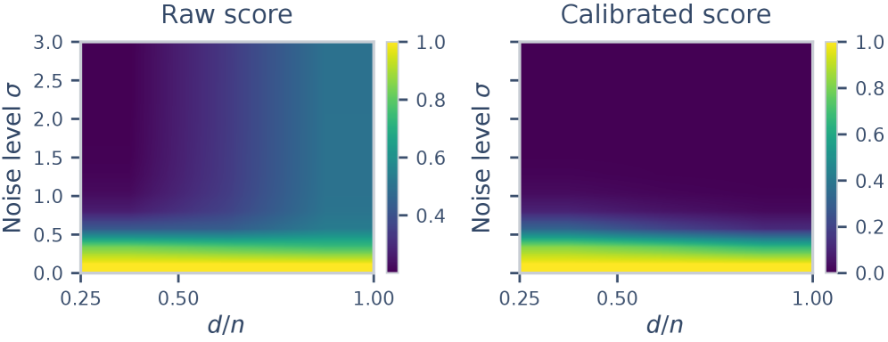
Figure 8 shows phase diagrams under different noise distributions: Gaussian, Student- $t$ ($\nu=3$), Laplace, and Gaussian mixtures. Each panel shows raw scores (left) and calibrated scores (right) across the $(d/n,\sigma)$ grid, where $\sigma$ controls the noise level added to a fixed shared signal. At low $\sigma$, the signal dominates and both raw and calibrated scores correctly indicate high similarity. At high $\sigma$, noise overwhelms the signal, and similarity should approach zero. The key finding is that raw scores remain elevated (around 0.4–0.6) even at high noise levels where no detectable signal remains, while calibrated scores correctly collapse to near-zero. This pattern holds across all noise distributions tested, confirming that permutation-based calibration adapts to the data-generating process without requiring explicit distributional modeling.

(a) Gaussian

F.2 SNR sweep heatmaps

The experiments of the main paper (Figure 4) demonstrated that calibration eliminates false positives under $H_{0}$ while preserving sensitivity to fixed signals. This section extends the analysis by characterizing how calibrated similarity varies jointly with signal strength, noise level, and dimensionality ratio, thereby delineating the regimes in which similarity estimation remains reliable.

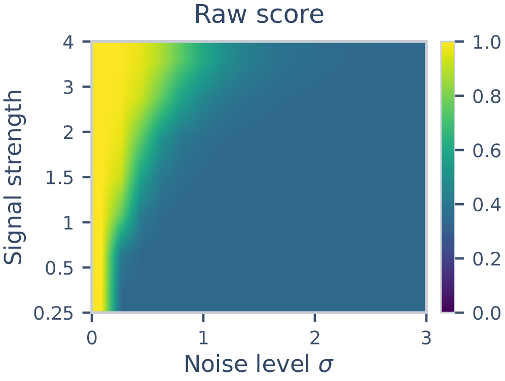
Figure 9 presents heatmaps of raw scores (top row) and calibrated scores (bottom row) across the (Noise level, Signal strength) grid for three signal ranks ($r\in{1,5,10}$). The results reveal a clear phase transition structure. Raw scores (top) show uniformly high values across most of the grid, obscuring the true detection boundary. Calibrated scores (bottom) reveal the underlying signal: high scores concentrate in the low-noise, high-signal corner (bottom-left), while scores correctly collapse to zero as noise increases (moving right) or signal weakens (moving down). The detection boundary shifts rightward (tolerating higher noise) as signal rank increases. This phase structure is meaningful: it delineates when similarity measurements carry information about shared structure versus when they reflect only finite-sample artifacts.

(a) Rank r = 1 r=1

Figure 10 provides a complementary view by collapsing the 2D heatmaps into 1D curves, plotting calibrated score against noise level for different signal strengths $s$. As expected, calibrated scores decrease monotonically with noise level: at low noise, scores are high (reflecting the detectable shared signal), while at high noise, scores collapse to zero (reflecting that the signal is buried). Stronger signals (larger $s$) maintain elevated scores across a wider range of noise levels before eventually succumbing. Higher-rank signals ($r=5,10$) show more gradual decay compared to $r=1$, consistent with their greater statistical detectability. All curves converge to zero at high noise, confirming that the null floor is correctly calibrated regardless of signal strength or rank.

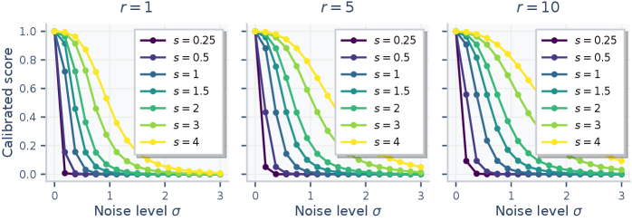
Figure 10: Calibrated scores decay with noise level. Each curve shows calibrated score versus noise level for a fixed signal strength s. Stronger signals maintain elevated scores across wider noise ranges; all curves converge to zero at high noise.

F.3 Comparing calibration approaches

A natural question is whether the choice of calibration summary affects the correction. We consider several approaches: (i) gated score, which thresholds at a significance level and rescales ($\alpha\in{0.05,0.1}$); (ii) null-centered, subtracting the null mean; (iii) z-score, standardizing by null mean and standard deviation; and (iv) ARI-style, applying the chance-correction formula $(s-\mathbb{E}[s])/(s_{\max}-\mathbb{E}[s])$. Figure 11 evaluates these variants across metrics as $d/n$ increases.

The results demonstrate that the gated score, null-centered, and ARI-style corrections all successfully collapse to appropriate null baselines across all metrics, regardless of whether the raw metric exhibits severe inflation (CKA, approaching 0.8) or mild inflation (RSA and mKNN, below 0.1). The z-score calibration, while correcting the mean, can exhibit artifacts when the null distribution is skewed, as occurs for bounded metrics like CKA at high $d/n$, making it less suitable as a universal correction.

(a) CKA linear

F.4 Comparison with analytical debiasing

We validate our empirical null calibration by comparing it to existing analytical bias corrections for CKA. Figure 12 shows the difference between our calibrated CKA and two existing estimators: the debiased CKA of ²⁰ and the dep-cols CKA of ²¹.

Our calibrated CKA closely matches the debiased CKA estimator, indicating that our calibration automatically corrects the dominant width-induced bias without requiring a metric-specific derivation. In contrast, dep-cols CKA is designed to correct column dependence, which is not a confound in our experimental setup (where columns are independent by construction), and as a result, it attenuates the true signal under $H_{1}$.

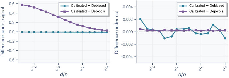
Figure 12: Calibration recovers analytical debiasing. Difference between calibrated CKA and existing estimators ( n = 1024 n=1024, d / d/n swept). (Left) Under signal. (Right) Under null.

F.5 Permutation budget analysis

Permutation-based calibration introduces a computational-statistical tradeoff: more permutations yield more stable threshold estimates but increase runtime. Practitioners need guidance on the minimum budget required for reliable inference.

We analyze the stability of threshold estimates $\tau_{\alpha}$ and calibrated scores as a function of the permutation budget $K$ across 50 random seeds. Figure 13 shows two panels: the left panel displays threshold estimates, while the right panel shows calibrated scores under $H_{0}$. Threshold estimates (left) stabilize rapidly, reaching stable values by approximately $K=50$ for all metrics tested. Calibrated scores (right) exhibit more variability at very low budgets ($K<50$), with occasional spikes due to unstable threshold estimation, but converge to near-zero by $K\approx 100$ – $200$.

Based on these results, we recommend $K\geq 200$. The computational cost scales linearly with $K$, so this recommendation represents a favorable tradeoff between precision and efficiency.

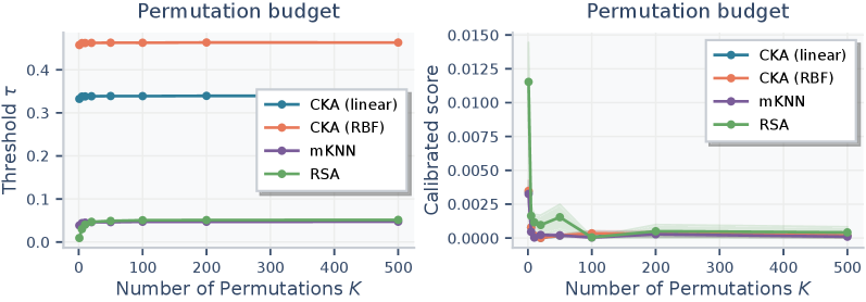
Figure 13: Permutation budget analysis. Left: threshold τ α \tau_{\alpha} stabilizes by K ≈ 50 K\approx 50. Right: calibrated scores under H 0 H_{0} converge to near-zero by 100 K\approx 100 – 200. Shaded regions show variability across random seeds.

F.6 Full null drift results

The main text presents null drift results for a representative subset of metrics under Gaussian noise. Here, we present additional results across all metrics evaluated in this work, including RSA, the RV coefficient, and Procrustes distance, as well as results under heavy-tailed noise distributions.

Figure 14 presents results under Gaussian noise for all metrics. The severity of null drift varies substantially across metric families: CKA variants exhibit the most severe inflation, followed by RV coefficient and CCA-variants, with neighborhood metrics showing the mildest drift. This reflects the structural sensitivity of the metrics to high-dimensional spurious correlations. Critically, calibration eliminates drift across all metrics, collapsing scores to zero regardless of the raw bias magnitude.

Figure 15 extends these results to heavy-tailed noise (Student- $t$, $\nu=3$). The qualitative pattern is preserved: all metrics exhibit positive drift under the null, and calibration eliminates this drift. The magnitude of raw bias is generally higher under heavy-tailed noise, consistent with increased finite-sample variability, yet calibration adapts automatically without requiring distributional knowledge.

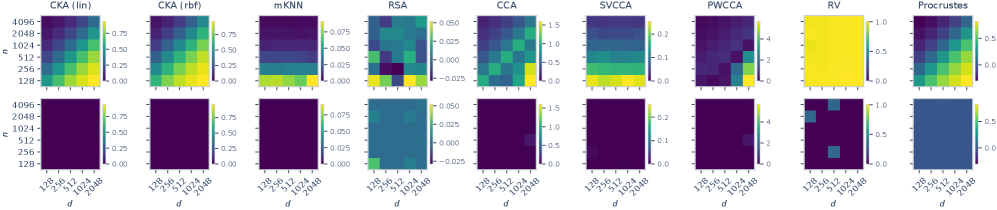
Figure 14: Full null drift results (Gaussian). Raw scores (top) exhibit systematic positive bias; calibrated scores (bottom) collapse to zero.

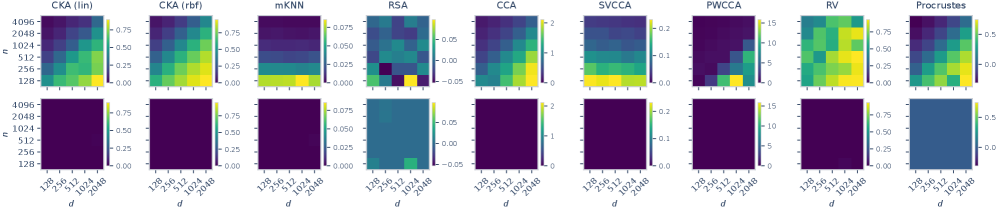
Figure 15: Full null drift results (heavy-tailed). Student- t ( ν = 3 \nu=3 ) noise. The pattern is consistent across all metrics: calibration eliminates spurious similarity regardless of noise distribution.

F.7 Extended PRH alignment results (image–text)

The main text establishes a divergence between local and global similarity metrics when applied to the Platonic Representation Hypothesis (PRH): neighborhood-based metrics retain significant cross-modal alignment after calibration, while spectral metrics lose their apparent convergence trend. A natural question is whether this finding is robust across model families and metric variants.

Here we present comprehensive results across all five vision model families in the PRH setting (DINOv2, CLIP, ImageNet-21K, MAE, and CLIP-finetuned) and a broad range of metrics spanning the local-to-global spectrum (Figures 16 and 17).

The results reinforce and extend the main text findings. Neighborhood metrics (mKNN, cycle- $k$ NN, CKNNA) show a consistent alignment trend across all vision families with a neighborhood size of 10. This pattern holds for both self-supervised (DINOv2, MAE) and supervised (ImageNet-21K) pretraining objectives, as well as for both CLIP-aligned and CLIP-finetuned variants. Spectral metrics (CKA linear, CKA RBF, unbiased CKA) show a different pattern: raw scores suggest increasing alignment with model scale, but calibrated scores show no such scaling trend.

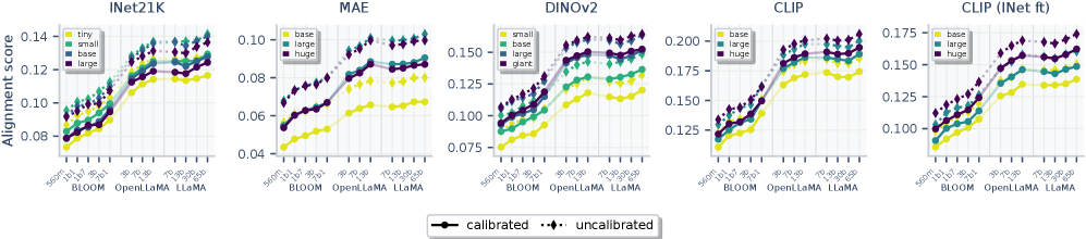
(a) mKNN: Neighborhood overlap.

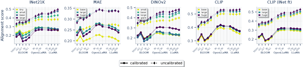
(a) CKA linear.

Statistical significance.

Beyond calibrated scores, we report permutation $p$ -values to quantify statistical evidence against the null hypothesis of no cross-modal alignment (Figure 18). All 204 vision–language model pairs are significant at $p<0.05$, with most achieving $p<0.005$ (the minimum achievable with $K=200$ permutations) for both local and global metrics. This confirms that cross-modal similarity is statistically significant (i.e., has some alignment) across all model pairs. The critical distinction between local and global metrics lies not in statistical significance but in the magnitude and trends of calibrated scores. Local metrics show substantial alignment above the null threshold that persists across scales, whereas global metrics, although significant, show no convergence in calibrated effect sizes.

(a) mKNN ( k = 10 k=10 ).

F.8 Extended video–language alignment results

The main text extends the PRH analysis to video–language alignment following ⁹. Here, we provide additional results to verify that the local-vs-global pattern observed for image–language alignment extends to the video modality.

We use 1024 samples from the PVD ^{44 45} test set. We evaluate both video-native models (VideoMAE ⁴⁶) and image models (DINOv2 and CLIP) applied to the middle frame of each video. We compare these against the same three language model families used in the image–language experiments (BLOOM, OpenLLaMA, LLaMA) at multiple scales. Figure 19 shows results for both spectral (CKA RBF) and neighborhood (mKNN) metrics.

The pattern mirrors the image–language findings. For spectral metrics, raw scores suggest alignment, whereas calibrated scores drop significantly, indicating that much of the apparent alignment is attributable to width and depth confounders. In contrast, neighborhood metrics retain significant alignment after calibration, confirming that video and language representations share local topological structure.

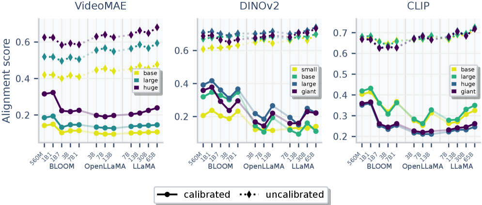
(a) CKA RBF: spectral alignment.

F.9 Characterizing the locality of cross-modal alignment

The main text establishes that local neighborhood metrics retain significant alignment after calibration, while global spectral metrics do not. A natural follow-up question is: how local is this alignment? Both mKNN and CKA -RBF have hyperparameters that control their sensitivity to local versus global structure. By varying these parameters, we can characterize the scale at which cross-modal alignment emerges.

Experimental setup.

We vary two locality parameters: the neighborhood size $k$ in mKNN, testing $k\in{10,20,50,100}$ where smaller values focus on immediate neighbors and larger values consider broader local structure, and the RBF kernel bandwidth $\sigma$ in CKA -RBF, testing $\sigma\in{0.1,0.5,2.0,5.0}$, which controls the length scale over which the kernel assigns significant weight.

RBF bandwidth.

The RBF (radial basis function) kernel is defined as $k(\mathbf{x},\mathbf{y})=\exp\left(-|\mathbf{x}-\mathbf{y}|^{2}/2\sigma^{2}\right)$. The bandwidth $\sigma$ determines the length scale of similarity. When $\sigma$ is small (e.g., $0.1$), the kernel is sharply peaked: only very close points contribute significantly to the Gram matrix, making the similarity measure sensitive to exact pairwise distances in the immediate neighborhood. When $\sigma$ is large (e.g., $5.0$), the kernel is broad: even moderately distant points contribute, and the similarity measure aggregates information over larger neighborhoods, becoming sensitive to coarser geometric structure.

Neighborhood size.

For mKNN, the parameter $k$ controls how many nearest neighbors are considered when measuring overlap. Small $k$ (e.g., $10$) measures agreement on immediate neighbors, i.e., the closest points to each sample, capturing fine-grained local topology. Large $k$ (e.g., $100$) measures agreement on a broader neighborhood. With $n=1000$ samples and $k=100$, we ask whether the $10\%$ closest points agree across representations. Crucially, mKNN is a rank-based metric: it asks which points are neighbors (ordinal information), not how close they are (cardinal information).

mKNN across kk values.

Figure 20 shows the PRH alignment results for mKNN with varying $k$. A consistent pattern emerges: all $k$ values show significant alignment after calibration, with calibrated scores remaining well above zero even at $k=100$. However, the scaling trend is most pronounced at small $k$. For $k=10$, raw scores show a clear upward trend with model capacity that persists after calibration. At large $k$, this trend flattens even in raw scores. For $k=100$, raw scores plateau for larger models, suggesting that broader neighborhood agreement is already saturated across model scales. This pattern indicates that scaling-driven improvement in alignment is concentrated at the finest topological level.

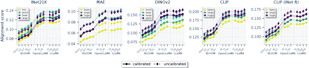
(a) mKNN ( k = 10 k=10 )

CKA-RBF across bandwidth values.

Figure 21, and the accompanying $p$ -values in Figure 22, shows results for CKA-RBF with varying bandwidth $\sigma$, revealing a different pattern from mKNN. At $\sigma=0.1$ (very local), there is no significant alignment after calibration: raw scores are near $1.0$, reflecting the high similarity of any high-dimensional representations under a sharply peaked kernel. However, calibrated scores collapse to approximately zero with $p$ -values exceeding $0.05$ for most model pairs, indicating that the observed similarity is indistinguishable from chance. At $\sigma=0.5$, alignment emerges, but with a flattening trend after calibration. Calibrated scores initially rise with model scale, then plateau and slightly decline for the largest models. At $\sigma=2.0$ and $\sigma=5.0$, significant alignment persists, but the calibrated trend also flattens, resembling the pattern observed for large- $k$ mKNN: alignment exists, but scaling-driven improvement disappears after calibration.

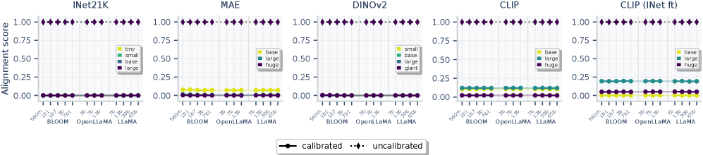
(a) CKA-RBF ( σ = 0.1 \sigma=0.1 )

(a) CKA-RBF ( σ = 0.1 \sigma=0.1 )

Topological versus metric alignment.

The contrasting behavior of mKNN and small- $\sigma$ CKA-RBF reveals a fundamental distinction in what “local alignment” means. On one hand, mKNN measures topological alignment: do the representations agree on which points are neighbors? This captures ordinal information where the ranking of distances matters but not their absolute values. On the other hand, small- $\sigma$ CKA-RBF measures metric alignment: do the representations agree on how close neighbors are? This captures cardinal information where exact distance values matter.

The fact that mKNN shows alignment at all $k$ values while small- $\sigma$ CKA-RBF shows no alignment reveals that cross-modal representations agree on neighborhood identity (which points are close) but not on exact local distances (how close they are). This finding is consistent with the observation that different training objectives and architectures induce different distance scales in representation space while preserving the relative ordering of neighbors. The Aristotelian Representation Hypothesis should therefore be understood as convergence to shared topological structure rather than shared metric structure.

F.10 Sensitivity to significance level α\alpha

The main text uses a significance level of $\alpha=0.05$ throughout. A natural concern is whether the conclusions of the PRH analysis depend on this particular choice. We repeat the PRH evaluation from Section 6.3 with $\alpha\in{0.01,0.05,0.10}$ for representative global (CKA linear, CKA RBF) and local (mKNN with $k=10$) metrics.

Figures 23, 24 and 25 show that the conclusions are entirely invariant to the choice of $\alpha$. For global metrics, calibrated scores show no convergence trend at any significance level. For local metrics, calibrated scores retain their alignment trend across all three $\alpha$ values. Stricter thresholds ($\alpha=0.01$) produce slightly lower calibrated scores, while more permissive thresholds ($\alpha=0.10$) produce slightly higher ones, but the qualitative pattern is unchanged. This confirms that our findings are not an artifact of a particular significance level.

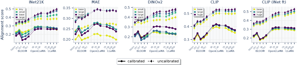
(a) α = 0.01 \alpha=0.01

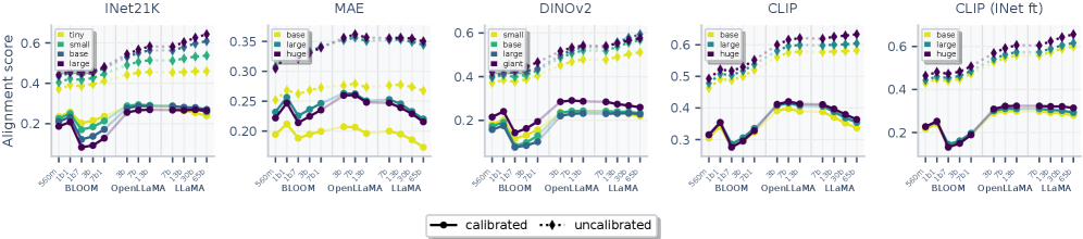
(a) α = 0.01 \alpha=0.01

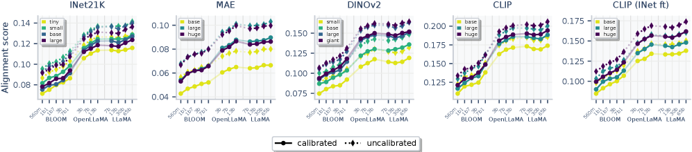
(a) α = 0.01 \alpha=0.01

1. SVCCA: Singular Vector Canonical Correlation Analysis for Deep Learning Dynamics and Interpretability. In Advances in Neural Information Processing Systems, Cited by: §C.2.1, §C.2.1, §1, §2. ↩ ↩² ↩³ ↩⁴

2. Do Wide and Deep Networks Learn the Same Things? Uncovering How Neural Network Representations Vary with Width and Depth. In International Conference on Learning Representations, Cited by: §1. ↩

3. Similarity of neural network representations revisited. In International Conference on Machine Learning, Cited by: §C.2.1, §C.2.1, §C.2.1, §C.2, §1, §2. ↩ ↩² ↩³ ↩⁴ ↩⁵ ↩⁶ ↩⁷

4. What is being transferred in transfer learning?. Advances in Neural Information Processing Systems. Cited by: §1. ↩

5. Brain-score: Which artificial neural network for object recognition is most brain-like?. BioRxiv. Cited by: §1, §1. ↩ ↩²

6. Position: The platonic representation hypothesis. In International Conference on Machine Learning, Cited by: §C.2.3, §C.2.3, §C.2.3, §C.2, §1, §1, §1, §2, §2, Figure 6, Figure 6, §6.3, §6.3. ↩ ↩² ↩³ ↩⁴ ↩⁵ ↩⁶ ↩⁷ ↩⁸ ↩⁹ ↩¹⁰ ↩¹¹ ↩¹² ↩¹³ ↩¹⁴

7. Do Vision and Language Encoders Represent the World Similarly?. In Conference on Computer Vision and Pattern Recognition, Cited by: §1, §1. ↩ ↩²

8. Understanding the Emergence of Multimodal Representation Alignment. In International Conference on Machine Learning, Cited by: §1, §1. ↩ ↩²

9. Dynamic Reflections: Probing Video Representations with Text Alignment. In International Conference on Learning Representations, Cited by: §F.8, §1, §2, §6.3. ↩ ↩² ↩³ ↩⁴

10. Canonical correlation analysis. In Proceedings of the Institute of Phonetic Sciences of the University of Amsterdam, Cited by: §C.2.1, §1. ↩ ↩²

11. Representational similarity analysis–connecting the branches of systems neuroscience. Frontiers in Systems Neuroscience. Cited by: §C.2.2, §C.2, §1, §2. ↩ ↩² ↩³ ↩⁴

12. Categories. Cited by: §1. ↩

13. Relations between two sets of variates. In Breakthroughs in Statistics: Methodology and Distribution, Cited by: §2. ↩

14. Insights on representational similarity in neural networks with canonical correlation. Advances in Neural Information Processing Systems. Cited by: §C.2.1, §C.2.1, §2. ↩ ↩² ↩³

15. Grounding representation similarity through statistical testing. Advances in Neural Information Processing Systems. Cited by: §2. ↩ ↩²

16. Generalized Shape Metrics on Neural Representations. In Advances in Neural Information Processing Systems, Cited by: §C.2.2, §2. ↩ ↩²

17. Similarity of neural network models: a survey of functional and representational measures. ACM Computing Surveys. Cited by: §2. ↩

18. What Representational Similarity Measures Imply about Decodable Information. In Proceedings of UniReps: the Second Edition of the Workshop on Unifying Representations in Neural Models, Cited by: §2. ↩

19. Evaluating representational similarity measures from the lens of functional correspondence. arXiv preprint arXiv:2411.14633. Cited by: §2. ↩

20. Correcting biased centered kernel alignment measures in biological and artificial neural networks. arXiv preprint arXiv:2405.01012. Cited by: Table 1, §F.4, §2, §6.1. ↩ ↩² ↩³ ↩⁴

21. Estimating Neural Representation Alignment from Sparsely Sampled Inputs and Features. arXiv preprint arXiv:2502.15104. Cited by: Table 1, §F.4, §2. ↩ ↩² ↩³

22. When is “nearest neighbor” meaningful?. In International Conference on Database Theory, Cited by: §2. ↩

23. On the surprising behavior of distance metrics in high dimensional space. In International Conference on Database Theory, Cited by: §2. ↩

24. Deconfounded representation similarity for comparison of neural networks. Advances in Neural Information Processing Systems. Cited by: Table 1, §2. ↩ ↩²

25. Resampling-based multiple testing: Examples and methods for p-value adjustment. John Wiley & Sons. Cited by: §2. ↩

26. Nonparametric permutation tests for functional neuroimaging: a primer with examples. Human Brain Mapping. Cited by: §2, §5.1. ↩ ↩²

27. Disentangling the factors of convergence between brains and computer vision models. arXiv preprint arXiv:2508.18226. Cited by: §2. ↩

28. Convergent transformations of visual representation in brains and models. arXiv preprint arXiv:2507.13941. Cited by: §2. ↩

29. The strong limits of random matrix spectra for sample matrices of independent elements. The Annals of Probability. Cited by: §4.1. ↩

30. A random matrix model of communication via antenna arrays. IEEE Transactions on information theory. Cited by: §4.1. ↩

31. Controlling the false discovery rate: a practical and powerful approach to multiple testing. Journal of the Royal Statistical Society. Cited by: §4.2, §5.2, §6.3. ↩ ↩² ↩³

32. Teoria statistica delle classi e calcolo delle probabilita. Pubblicazioni del R istituto superiore di scienze economiche e commericiali di firenze. Cited by: §4.2. ↩

33. Permutation P-values Should Never Be Zero: Calculating Exact P-values When Permutations Are Randomly Drawn.. Statistical Applications in Genetics & Molecular Biology. Cited by: §D.1, §5.1. ↩ ↩²

34. Permutation, parametric and bootstrap tests of hypotheses. Springer. Cited by: §5.1. ↩

35. A simple sequentially rejective multiple test procedure. Scandinavian Journal of Statistics. Cited by: §5.2. ↩

36. Wit: wikipedia-based image text dataset for multimodal multilingual machine learning. In International ACM SIGIR Conference on Research and Development in Information Retrieval, Cited by: §6.3. ↩

37. Comparing representational geometries using whitened unbiased-distance-matrix similarity. arXiv preprint arXiv:2007.02789. Cited by: Table 1. ↩

38. Representational structure or task structure? Bias in neural representational similarity analysis and a Bayesian method for reducing bias. PLoS Computational Biology. Cited by: Table 1. ↩

39. Matrix correlations for high-dimensional data: the modified RV-coefficient. Bioinformatics. Cited by: Table 1, §C.2.1. ↩ ↩²

40. Feature Selection via Dependence Maximization. Journal of Machine Learning Research. Cited by: §C.2.1. ↩

41. A unifying tool for linear multivariate statistical methods: the RV-coefficient. Journal of the Royal Statistical Society. Cited by: §C.2.1. ↩

42. Mathematical methods of statistics. Princeton University Press. Cited by: §D.5. ↩

43. Modelling extremal events: for insurance and finance. Springer Science & Business Media. Cited by: §D.5. ↩

44. Perception encoder: the best visual embeddings are not at the output of the network. Advances in Neural Information Processing Systems. Cited by: §F.8. ↩

45. PerceptionLM: open-access data and models for detailed visual understanding. Advances in Neural Information Processing Systems. Cited by: §F.8. ↩

46. VideoMAE: Masked autoencoders are data-efficient learners for self-supervised video pre-training. Advances in Neural Information Processing Systems. Cited by: §F.8. ↩